Abstract
Currently, FEA software such as ABAQUS uses empirical models to predict the sound absorption coefficient of poroelastic materials. However, based on a recent review of the literature it was found that the current sound absorption empirical models are inadequate for accurate prediction of thin (t< 20 mm), low-density materials (ρB < 50 kg/m3). Therefore, the predictions of the sound pressure levels in vehicle cabins, using such software, will be inaccurate since the trim materials are thin and have a low density. Thus, this research aimed to develop an empirical model that can accurately predict the sound absorption coefficient of these materials. Hence, polypropylene fibres consisting of four different diameters were manufactured and converted into nonwovens. Thereafter, airflow resistivity and impedance tube experimental testing were performed on the specimens. Subsequently, statistical analysis of the data was performed using SAS software. SAS was used to identify which independent variables should be included in the models to be developed. The empirical models were developed using the regression analysis toolbox in Microsoft Excel. Once the models were developed, various checks were performed to validate the assumptions of linear regression. The software NumXL was used to perform Cook’s distance tests. Thereafter, the models were validated against the validation dataset, where it was found that the developed exponential model performed best. Finally, the exponential model was compared to existing models using two data sets i.e. an internal dataset, and an external dataset derived from the literature. The developed model outperformed all the historic models on both datasets.
Highlights
- Current Limitations: Traditional empirical sound absorption models fail to accurately predict the behavior of thin, low-density fibrous acoustic materials.
- Innovative Approach: An empirical exponential model has been developed, offering precise sound absorption predictions within the low to mid-frequency spectrum.
- Key Parameters: The model incorporates material thickness, bulk density, and fibre diameter as predictors.
- Superior Performance: Comparative analysis demonstrates that the new model consistently surpasses established models in predicting the sound absorption coefficient, validated by both internal and external datasets.
- Simplified Methodology: The innovative model eliminates the need for airflow resistivity measurements, streamlining the prediction process.
1. Introduction
Current analytical models for the prediction of the sound absorption coefficient can provide accurate results over large operating ranges, but they are highly complex and require comprehensive experimental testing to determine many variables [1]. This is often not feasible to use in practical applications [2]. Empirical models on the other hand offer the advantage of simplicity. The development of empirical models for this purpose is therefore not new and dates to the 1970s when Delany and Bazley presented the first empirical model for fibrous sound absorbers. This power-law function model provided a simpler method of relating the complex relationship between airflow resistivity, surface characteristic impedance, frequency, and the propagation wavenumber in order to predict the sound absorption coefficient of a fibrous material [3]. Many similar models have since been proposed for a variety of different fibres, natural and synthetic i.e., Mechel, Miki, Garai, Del Rey, Komatsu, Egab, Ramis, Liu, and Berardi models, refer to Table 8 for references. Each new model developed catered for a different range of material thickness, bulk density, and fibre diameter. All the variant models developed except for the Voronina model [4], and the Allard and Champoux model [5], used the same formulation with only the coefficients being adapted for new materials.
It must be noted that empirical models do however have their limitations. They may fail to accurately predict the sound absorption coefficient of absorbing materials in certain ranges. Reasons for this include inadequate pre-processing of the data, inadequate model validation, unjustified extrapolation (e.g., application of the model to data that reside in a space which the model has never seen), or, most importantly, over-fitting the model to the existing data [6]. With this said caution should always be exercised when selecting an empirical model for real-world application.
The idea for this research topic stemmed from a paper by Dunne et al [7]. In this research, a review of all the existing empirical models for the prediction of the sound absorption coefficients was given. After reviewing the current models, the paper went on to test the model prediction accuracies over the working ranges of these models. These results are summarised in Fig. 1.
Fig. 1Sound absorption model accuracy for empirical models [7]
![Sound absorption model accuracy for empirical models [7]](https://static-01.extrica.com/articles/23978/23978-img1.jpg)
Fig. 1, demonstrates that the current available empirical models for the prediction of the sound absorption coefficient, of thin, low-density poroelastic materials, are inadequate. The range in which the current sound absorption coefficient models are not accurate correspond to densities less than 50.0 kg/m3 and thicknesses lower than 20.0 mm. This poses a problem for Finite Element Analysis (FEA) users, modelling thin low-density materials, such as those applied in vehicles for noise mitigation, since such software often employs empirical models for prediction. Since the FEA software is only as accurate as the models it utilises for prediction, it is necessary to develop a model that can accurately predict the sound absorption coefficient for this range of materials.
Therefore, this paper aims at developing a simple empirical model using multiple linear regression analysis. The model should be able to accurately predict the sound absorption coefficient of low-density, less than 50 kg/m3, thin, less than 20 mm thick, fibrous materials in the low to mid-frequency range (100-2000 Hz). Furthermore, an attempt will be made to develop a model with parameters that don't require experimental testing.
2. Equipment and measurements
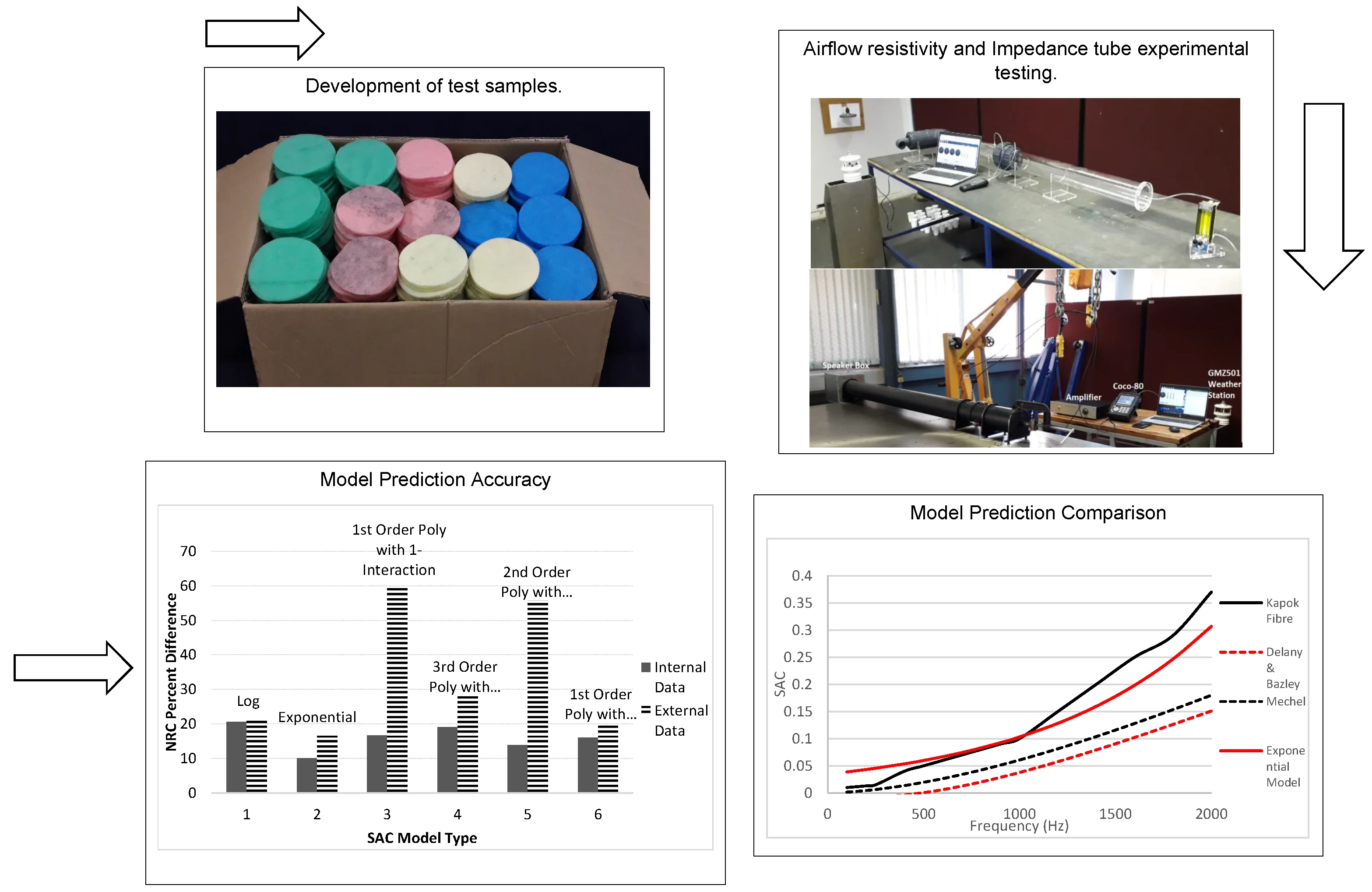
The experimental testing done for this research was performed on equipment that was designed according to the ISO standards 9053-1 and 10534-2. Manufacturing of the experimental equipment was produced according to the specifications set out in the ISO standards and was of high quality. Two devices were developed to perform experimental measurements. The first was an airflow resistivity apparatus and the second was an impedance tube. The airflow resistivity tube was used to test the airflow resistance and the impedance tube was used to test the sound absorption, of various fibrous materials. It was necessary to quantify the airflow resistivity of the various materials since this is one of the parameters that the sound absorption coefficient has been shown to be dependent on.
The fibres developed for this research were manufactured from polypropylene copolymer (HSV103). The polypropylene fibres were manufactured to four different diameters; yellow – 19.4 μm, red – 29.7 μm, green – 40.8 μm and blue – 49.5 μm. This was done since the airflow resistivity of fibrous materials is dependent on the fibre diameter. Each fibre was coloured differently for identification purposes. Thereafter, the fibres were manufactured into nonwovens using an Aolong Nonwoven Needlepunching Machine. Specimens of 100 mm diameter were then cut out of the various nonwovens using a laser cutting machine. The total number of samples used in this research for the development and validation of the empirical model was 203 samples. The number of samples that were used for the model development dataset was 180 and the number of samples that were used as the validation dataset was 23. The software G*Power was utilised to check the required minimum number of samples that should be used for model development [8]. The number of samples utilised in this research was far higher than the necessary minimum number.
2.1. Thickness and bulk density experimental measurements and results
The mass of each sample was determined using a calibrated KERN PFB 2000-2 scale with an accuracy of 0.01 g and precision of ±0.03 g. Thereafter, the volume of each sample was calculated using the dimensions of the sample which were measured using a vernier calliper. From the mass and the volume, the bulk density of each sample was then determined and presented in Tables 1-4.
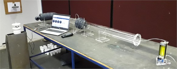
2.2. Airflow resistivity experimental measurements
The airflow resistivity tube presented in Fig. 2 was designed, developed and calibrated according to the ISO 9053-1 first edition 2018-10. The tube was manufactured from poly (methyl methacrylate) also known as plexiglass or acrylic glass. The air supply to the device was obtained from a central air compressing unit and was filtered before use. A pressure regulator to regulate the pressure coming into the flow meter was attached to the inlet line. A testo 512 pressure meter (0-200 Pa), with a resolution of 0.1 Pa, was used to measure the differential pressure as required by the ISO standard. A KOFLOC flow meter model RK120X series was used to regulate the inlet flow. This flow meter can measure flows as low as 5 ml/min, which is far lower than what is required by the ISO standard. A MaxiMet (GMX501) Compact Weather Station was utilised to monitor the ambient temperature, pressure and humidity in the laboratory where testing was conducted. The MaxiMet Compact Weather Station provides pressure (accuracy of 0.1 hPa), temperature (accuracy of 0.1 °C) and accurate humidity data.
Table 1Specimen properties of 19.4 μm diameter fibre
Sample No. | Thickness (mm) | Bulk density (kg/m3) | Porosity | Airflow resistivity (Pa.s/m2) | NRC |
Y56 | 10.5 | 20.62 | 0.977 | 7029.629 | 0.15 |
Y53 | 11.6 | 21.92 | 0.976 | 7545.725 | 0.17 |
Y55 | 8.9 | 22.49 | 0.975 | 8444.663 | 0.11 |
Y54 | 8.5 | 22.58 | 0.975 | 7492.902 | 0.18 |
Y60 | 8.2 | 23.11 | 0.974 | 9181.513 | 0.15 |
Y59 | 8.4 | 24.95 | 0.972 | 10053.372 | 0.14 |
Y57 | 13.1 | 25.07 | 0.972 | 10043.68 | 0.17 |
Y51 | 8.7 | 26.25 | 0.971 | 8144.818 | 0.21 |
Y41 | 9 | 26.55 | 0.971 | 10075.121 | 0.15 |
Y52 | 8.4 | 27.33 | 0.97 | 9199.771 | 0.13 |
Y6 | 9.3 | 27.47 | 0.97 | 10134.17 | 0.17 |
Y58 | 10.7 | 27.72 | 0.969 | 10158.223 | 0.15 |
Y24 | 7.7 | 28.13 | 0.969 | 9624.715 | 0.16 |
Y42 | 10.2 | 28.97 | 0.968 | 9603.044 | 0.16 |
Y21 | 8.2 | 29.72 | 0.967 | 10838.636 | 0.15 |
Y8 | 11.4 | 31.08 | 0.966 | 10045.336 | 0.17 |
Y40 | 8.5 | 31.58 | 0.965 | 10232.096 | 0.17 |
Y5 | 10.9 | 32.29 | 0.964 | 9673.632 | 0.18 |
Y9 | 12.2 | 32.61 | 0.964 | 12135.436 | 0.17 |
Y43 | 9.4 | 32.81 | 0.964 | 11854.76 | 0.16 |
Y10 | 8.5 | 33.52 | 0.963 | 12629.01 | 0.15 |
Y7 | 8.6 | 33.81 | 0.963 | 12581.789 | 0.14 |
Y12 | 10.2 | 34.05 | 0.962 | 11227.14 | 0.16 |
Y34 | 9.4 | 34.31 | 0.962 | 12854.285 | 0.17 |
Y20 | 11.6 | 34.81 | 0.962 | 13513.737 | 0.18 |
Y19 | 10.8 | 35.97 | 0.96 | 13711.948 | 0.16 |
Y18 | 11.3 | 38.55 | 0.957 | 14423.639 | 0.17 |
Y3 | 12 | 38.85 | 0.957 | 15667.163 | 0.17 |
Y2 | 13.3 | 38.94 | 0.957 | 15194.283 | 0.2 |
Y50 | 11.4 | 39.76 | 0.956 | 15799.167 | 0.2 |
Y49 | 10.7 | 40.16 | 0.956 | 14760.509 | 0.18 |
Y37 | 11.4 | 40.17 | 0.956 | 14954.269 | 0.17 |
Y27 | 10.9 | 40.61 | 0.955 | 16568.816 | 0.17 |
Y29 | 10.7 | 40.82 | 0.955 | 14524.575 | 0.18 |
Y45 | 9.6 | 42.06 | 0.954 | 15769.624 | 0.17 |
Y15 | 9 | 43.82 | 0.952 | 13154.191 | 0.13 |
Y35 | 10.7 | 44.01 | 0.951 | 16088.508 | 0.19 |
Y1 | 12.2 | 44.29 | 0.951 | 19264.355 | 0.2 |
Y30 | 12.1 | 44.36 | 0.951 | 19186.155 | 0.19 |
Y26 | 11.9 | 46.49 | 0.949 | 18346.929 | 0.18 |
Y44 | 9.9 | 47.44 | 0.948 | 21000.789 | 0.19 |
Y47 | 11.2 | 47.93 | 0.947 | 21282.25 | 0.2 |
Y31 | 11.5 | 49.44 | 0.945 | 23797.372 | 0.21 |
Y61 | 11 | 49.76 | 0.945 | 23648.788 | 0.18 |
Y17 | 12.5 | 50.76 | 0.944 | 23843.627 | 0.24 |
The experimental testing began by preparing the local environment (the laboratory) for testing. This was achieved by ensuring that the lab temperature was constant. Hence, the air conditioning units in the laboratory were turned on at a temperature of 22 °C several hours before testing began. This allowed for the temperature of the room to stabilise. The order of testing for the specimens was random. This is important in order to eliminate the effect of any nuisance variable that may influence the observed airflow resistivity [9]. Therefore, since the testing was randomized and the environment, in which tests were performed, was as uniform as possible, this experimental design is a completely randomized design. The airflow resistivity of each sample is presented in Tables 1-4.
Fig. 2Airflow resistivity experimental setup
2.3. Sound absorption coefficient experimental measurements and results
Before the testing commenced the laboratory environment was given enough time for the ambient temperature to stabilise to approximately 22 °C. This temperature was maintained by using two air conditioning units. All experimental testing was carried out over a three-day period. The laboratory temperature, pressure, and humidity were monitored and captured for each test using the GMX501 Compact weather station. The temperature in the laboratory fluctuated no more than 2 °C during the three-day testing period. Microphone amplitude and phase calibration tests were performed according to the ISO 10534-2 standard. Furthermore, a reference test was performed using a manufacturer's sample. This was done to validate that the impedance tube using the two-microphone transfer function method was indeed capturing the data accurately. The setup is illustrated in Fig. 3.
Fig. 3Assembled impedance tube
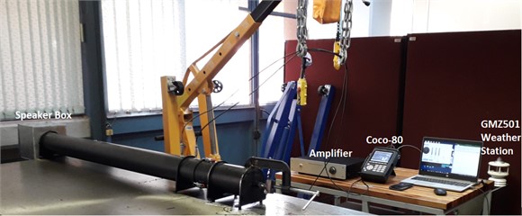
Once the experimental setup was ready testing proceeded. The data was captured utilising a Coco-80 dynamic signal analyser and saved to an SD card. The noise source used was a 2426H JBL professional series compression driver speaker. The microphones used were ICP with model number 130E20. The captured data was then downloaded from the SD card into the Engineering Data management (EDM) software, where it was converted into excel format in order to be post-processed in MatLab using code that was developed for this research. The data for the sound absorption coefficient of the tested materials are presented in Table 1-4, in terms of the Noise Reduction Coefficient (NRC), for brevity. Also, it should be noted that all measurements below 100 Hz, were removed from the data set due to inaccuracies observed in the data below this frequency limit. The reason for these inaccuracies occurring in the data below 100 Hz are most likely due to the spacing between the microphones on the tube. This is because the measurement frequency range is dependent on the microphone spacing. As the spacing between the microphones reduces the accuracy of low-frequency measurements is limited but the accuracy of high-frequency measurements is improved.
Table 2Specimen properties of 29.7 μm diameter fibre
Sample No. | Thickness (mm) | Bulk density (kg/m3) | Porosity | Airflow resistivity (Pa.s/m2) | NRC |
R62 | 11.7 | 21.43 | 0.976 | 4181.467 | 0.11 |
R61 | 12 | 21.58 | 0.976 | 4076.93 | 0.15 |
R72 | 10.3 | 22.52 | 0.975 | 4136.866 | 0.13 |
R75 | 10.3 | 24.12 | 0.973 | 5325.411 | 0.15 |
R67 | 11.3 | 26.46 | 0.971 | 4880.613 | 0.13 |
R38 | 11.5 | 26.51 | 0.971 | 5353.834 | 0.14 |
R43 | 9.5 | 27.14 | 0.97 | 5615.964 | 0.12 |
R65 | 10.9 | 27.22 | 0.97 | 5350.34 | 0.14 |
R76 | 10.4 | 27.39 | 0.97 | 5737.029 | 0.12 |
R69 | 11.4 | 27.47 | 0.97 | 5400.798 | 0.14 |
R64 | 12 | 28.25 | 0.969 | 5992.259 | 0.13 |
R78 | 12.9 | 28.47 | 0.969 | 4864.124 | 0.15 |
R73 | 10.4 | 28.86 | 0.968 | 5220.59 | 0.14 |
R45 | 9.3 | 28.99 | 0.968 | 5067.085 | 0.13 |
R68 | 10.5 | 29.04 | 0.968 | 5352.203 | 0.14 |
R54 | 9 | 31.78 | 0.965 | 5683.162 | 0.12 |
R49 | 8.5 | 34.21 | 0.962 | 6047.986 | 0.14 |
R46 | 8.9 | 34.65 | 0.962 | 5843.287 | 0.13 |
R63 | 9.4 | 34.81 | 0.962 | 6438.5 | 0.15 |
R71 | 10.6 | 34.87 | 0.961 | 5857.501 | 0.14 |
R59 | 8.1 | 35.75 | 0.96 | 5506.098 | 0.14 |
R51 | 10.2 | 35.78 | 0.96 | 6430.752 | 0.14 |
R19 | 11.5 | 36.44 | 0.96 | 6609.939 | 0.16 |
R44 | 7.1 | 36.64 | 0.96 | 6001.369 | 0.15 |
R70 | 10.8 | 37.06 | 0.959 | 6473.837 | 0.14 |
R41 | 11.6 | 37.75 | 0.958 | 6198.889 | 0.16 |
R21 | 11.6 | 38.06 | 0.958 | 6735.765 | 0.17 |
R47 | 8.1 | 38.8 | 0.957 | 7329.124 | 0.14 |
R31 | 11.3 | 38.86 | 0.957 | 7389.898 | 0.16 |
R48 | 9 | 39.76 | 0.956 | 7884.959 | 0.15 |
R27 | 11.1 | 40.94 | 0.955 | 7039.178 | 0.14 |
R4 | 11.9 | 41.45 | 0.954 | 7894.839 | 0.15 |
R20 | 14.3 | 41.9 | 0.954 | 8156.462 | 0.17 |
R18 | 10.6 | 42.65 | 0.953 | 8764.281 | 0.15 |
R37 | 14.2 | 43.11 | 0.952 | 8076.418 | 0.16 |
R7 | 12.3 | 43.74 | 0.952 | 8509.627 | 0.16 |
R57 | 8.2 | 43.93 | 0.951 | 8218.652 | 0.15 |
R39 | 11.5 | 44.43 | 0.951 | 9360.503 | 0.16 |
R40 | 9 | 44.99 | 0.95 | 8481.733 | 0.13 |
R5 | 11.5 | 46.47 | 0.949 | 9542.625 | 0.14 |
R32 | 15.2 | 46.85 | 0.948 | 9897.757 | 0.21 |
R55 | 8.7 | 46.95 | 0.948 | 9478.005 | 0.14 |
R26 | 10.6 | 47.53 | 0.947 | 8764.281 | 0.15 |
R50 | 11.5 | 50.36 | 0.944 | 10333.965 | 0.16 |
R33 | 9.1 | 50.58 | 0.944 | 10397.25 | 0.15 |
Table 3Specimen properties of 40.8 μm diameter fibre
Sample No. | Thickness (mm) | Bulk density (kg/m3) | Porosity | Airflow resistivity (Pa.s/m2) | NRC |
G4 | 10.7 | 24.64 | 0.973 | 2004.407 | 0.11 |
G6 | 13.8 | 25.16 | 0.972 | 1554.141 | 0.14 |
G18 | 8.4 | 25.23 | 0.972 | 2198.783 | 0.13 |
G8 | 13.4 | 25.48 | 0.972 | 2502.648 | 0.14 |
G1 | 12 | 25.51 | 0.972 | 2136.668 | 0.12 |
G27 | 8.3 | 25.95 | 0.971 | 2364.551 | 0.09 |
G48 | 11.8 | 26.64 | 0.971 | 3083.217 | 0.13 |
G3 | 13 | 28.07 | 0.969 | 3690.822 | 0.13 |
G16 | 7 | 28.08 | 0.969 | 3732.803 | 0.09 |
G69 | 11.3 | 28.34 | 0.969 | 3619.126 | 0.13 |
G10 | 9.6 | 28.69 | 0.968 | 3789.787 | 0.11 |
G47 | 12.5 | 28.91 | 0.968 | 3340.234 | 0.12 |
G2 | 12.1 | 29.38 | 0.968 | 3965.346 | 0.13 |
G23 | 9.7 | 30.1 | 0.967 | 3750.717 | 0.12 |
G9 | 12.4 | 30.47 | 0.966 | 3869.41 | 0.15 |
G13 | 9.5 | 31.35 | 0.965 | 3620.24 | 0.13 |
G72 | 12.3 | 31.87 | 0.965 | 3721.747 | 0.14 |
G11 | 12.8 | 32.01 | 0.965 | 3995.973 | 0.13 |
G28 | 9 | 32.31 | 0.964 | 2848.891 | 0.14 |
G5 | 11.2 | 33.64 | 0.963 | 3502.538 | 0.15 |
G51 | 12.2 | 34.45 | 0.962 | 4166.161 | 0.15 |
G25 | 9.2 | 34.55 | 0.962 | 3630.933 | 0.15 |
G12 | 11.9 | 35.51 | 0.961 | 4199.19 | 0.14 |
G50 | 13.6 | 36.1 | 0.96 | 4055.216 | 0.15 |
G54 | 11.7 | 36.83 | 0.959 | 4027.683 | 0.14 |
G30 | 13 | 37.13 | 0.959 | 4176.472 | 0.14 |
G29 | 14 | 37.92 | 0.958 | 3939.352 | 0.14 |
G26 | 7 | 38.17 | 0.958 | 4430.141 | 0.13 |
G78 | 13.5 | 38.19 | 0.958 | 4560.674 | 0.15 |
G49 | 11.3 | 39.27 | 0.957 | 4973.286 | 0.16 |
G41 | 13.8 | 42.57 | 0.953 | 4883.547 | 0.15 |
G32 | 12 | 43.95 | 0.951 | 5378.872 | 0.14 |
G46 | 13.3 | 44.17 | 0.951 | 5660.782 | 0.15 |
G20 | 9 | 44.21 | 0.951 | 6348.956 | 0.13 |
G52 | 10.8 | 44.91 | 0.95 | 6862.065 | 0.14 |
G33 | 11.8 | 45.49 | 0.95 | 5845.335 | 0.14 |
G73 | 13.8 | 45.98 | 0.949 | 6924.453 | 0.15 |
G56 | 10.3 | 46.06 | 0.949 | 7195.175 | 0.13 |
G55 | 9.4 | 46.71 | 0.948 | 5584.559 | 0.13 |
G37 | 11 | 46.98 | 0.948 | 5963.061 | 0.14 |
G76 | 12.7 | 47.37 | 0.948 | 7367.161 | 0.18 |
G24 | 8.8 | 47.49 | 0.948 | 6169.788 | 0.15 |
G15 | 9.5 | 47.83 | 0.947 | 5615.964 | 0.14 |
G65 | 10.6 | 48.53 | 0.946 | 6864.52 | 0.14 |
G84 | 12.9 | 50.46 | 0.944 | 6473.321 | 0.16 |
3. Sound absorption coefficient model development
A model is simply the mathematical relationship between a predictor variable and a response variable. However, when no theoretical knowledge of the relationship between an independent variable x and dependent variable y is available the choice of the model implemented is based on an inspection of the scatter plots. From the analysis of these plots, it can be determined if the data falls on a straight line, show evidence of curvature, or indicate some anomaly [10]. Thereafter it can be determined if the method of least-squares can be implemented to develop regression models. These types of regression models are thought of as empirical models [9]. Since this was the case with the research being conducted, an empirical model approach was implemented. It must be noted at this point that the power law relationship proposed by Delany and Bazley was not utilised in this research. The reason for this was to develop a model with a simpler formation that did not require prior rigorous experimental testing of the parameters utilised in the model.
Table 4Specimen properties of 49.5 μm diameter fibre
Sample No. | Thickness (mm) | Bulk density (kg/m3) | Porosity | Airflow resistivity (Pa.s/m2) | NRC |
B51 | 12.8 | 20.32 | 0.978 | 1023.344 | 0.1 |
B50 | 10 | 20.95 | 0.977 | 1489.809 | 0.1 |
B40 | 11.4 | 20.96 | 0.977 | 1869.847 | 0.09 |
B25 | 11.4 | 22.2 | 0.975 | 1702.829 | 0.09 |
B32 | 8.6 | 23.27 | 0.974 | 1816.663 | 0.09 |
B23 | 11.5 | 24.06 | 0.973 | 1515.007 | 0.11 |
B54 | 12.2 | 24.8 | 0.973 | 1868.323 | 0.11 |
B33 | 10.4 | 25.13 | 0.972 | 2209.995 | 0.1 |
B55 | 9 | 26.29 | 0.971 | 2332.697 | 0.11 |
B26 | 9.8 | 26.67 | 0.971 | 2432.729 | 0.11 |
B24 | 12.3 | 26.89 | 0.97 | 2451.56 | 0.12 |
B44 | 10.5 | 27.02 | 0.97 | 2600.735 | 0.1 |
B53 | 7.3 | 27.09 | 0.97 | 2530.106 | 0.08 |
B27 | 7.5 | 27.78 | 0.969 | 2642.156 | 0.09 |
B37 | 14 | 30.19 | 0.967 | 2982.352 | 0.13 |
B29 | 10.4 | 31.92 | 0.965 | 2808.818 | 0.11 |
B42 | 10 | 32.37 | 0.964 | 2816.451 | 0.1 |
B28 | 9.9 | 32.82 | 0.964 | 2844.9 | 0.12 |
B30 | 12.8 | 33.11 | 0.963 | 2842.34 | 0.12 |
B36 | 11 | 33.28 | 0.963 | 2941.58 | 0.12 |
B46 | 10.4 | 33.84 | 0.963 | 3111.287 | 0.12 |
B49 | 8.7 | 34.5 | 0.962 | 2641.833 | 0.1 |
B43 | 10.3 | 34.97 | 0.961 | 3172.688 | 0.12 |
B31 | 11 | 35.1 | 0.961 | 3307.45 | 0.12 |
B39 | 8.5 | 35.18 | 0.961 | 2915.673 | 0.12 |
B47 | 11 | 35.42 | 0.961 | 3036.78 | 0.13 |
B52 | 12 | 36.3 | 0.96 | 3479.41 | 0.13 |
B41 | 8.5 | 37.39 | 0.959 | 3547.552 | 0.11 |
B45 | 9.2 | 38.77 | 0.957 | 4170.829 | 0.1 |
B19 | 9.5 | 40.52 | 0.955 | 3174.125 | 0.12 |
B34 | 8.2 | 41.2 | 0.954 | 3562.404 | 0.1 |
B11 | 9.7 | 41.5 | 0.954 | 3247.483 | 0.1 |
B16 | 9.1 | 41.65 | 0.954 | 3095.002 | 0.12 |
B20 | 9.8 | 42.52 | 0.953 | 3616.273 | 0.11 |
B35 | 8.3 | 42.55 | 0.953 | 3898.48 | 0.12 |
B17 | 10.8 | 44.25 | 0.951 | 3756.928 | 0.11 |
B48 | 8.5 | 44.59 | 0.951 | 4280.23 | 0.12 |
B21 | 10.3 | 45.83 | 0.949 | 4053.682 | 0.12 |
B57 | 11.4 | 46.36 | 0.949 | 4486.707 | 0.14 |
B8 | 10.8 | 47.31 | 0.948 | 4238.657 | 0.13 |
B15 | 10.5 | 48.32 | 0.947 | 4487.99 | 0.12 |
B10 | 8.5 | 48.89 | 0.946 | 4179.43 | 0.13 |
B38 | 9 | 49.31 | 0.946 | 4192.039 | 0.12 |
B5 | 9.9 | 49.82 | 0.945 | 4759.989 | 0.13 |
B13 | 9 | 50.62 | 0.944 | 4639.214 | 0.12 |
A regression model that contains more than one independent variable is called a multiple regression model. This is true for the model developed in this work and thus multiple linear regression was the tool used to develop the model. Building a regression model is an iterative process. It must be noted that designed experiments are the only way to determine cause-and-effect relationships between the model predictors and dependent variables [9]. A useful tool for this is Analysis of Variance (ANOVA), which helps determine the quality of the relationship between the response and predictor variables by evaluating the sum of square errors, the mean square error, F-values (indicates if the linear regression model provides a better fit to the data than a model that contains no independent variables) and the p-values (smallest choice of the significance level that would allow the null hypothesis to be rejected). Other criteria that can be used to evaluate the goodness of fit of the model are the adjusted R-squared value (goodness of fit measure) and information criteria. Furthermore, scatter plots of the residuals aid as a useful visual tool when examining the performance of the regression model. Lastly, this point is vital in the model development process and must be noted. Predictor variables with a weak or no correlation with the response variable may sometimes be excluded. Typically, the decision to discard a variable is based on the analysis tools, utilised in multiple regression analysis, as discussed above i.e. ANOVA, adjusted R-squared value and information criteria [11].
An important part of model building involves the selection of the regressor variables to be used in the model. This is done by screening all the possible variables to obtain a regression model that contains the best subset of regressor variables [11]. The use of good model selection techniques was implemented in this research in order to increase confidence in the variables selected for the final model.
Also, an essential part of the model-building process involves trying to identify some form of the equation that will fit the data best when there is curvature in the plot [10]. It must be noted that curvature was observed in some of the scatter plots, not included in this paper for the sake of brevity. However, the curvature was eliminated through the utilization of transformations which allowed for the linearization of the data since in order to apply the method of least-squares, for regression model development, the equations chosen must be linear in their coefficients. This is shown later in the model derivation section.
3.1. Sound absorption coefficient collinearity check
A collinearity analysis was performed on the sound absorption coefficient data using Statistical Analysis System (SAS) software [12]. As can be seen from Table 5, all the predictor variables had a Variance Inflation Factor (VIF) of less than 10, hence no collinearity was detected. This is important since collinearity occurs when there is a correlation present among predictor variables in the model. If the predictor variables are not correlated, then there's no collinearity present in the model. Collinear predictors provide redundant information and therefore cause instability in the model by inflating the variance of the parameter estimates, which raises the p-values. Hence, it is necessary to check for collinearity between predictors and remove redundancies.
Table 5Sound absorption coefficient collinearity check
Variable | DF | Parameter estimate | Standard error | t value | Pr > |t| | Variance inflation |
Intercept | 1 | –0.0714 | 0.00512 | –13.95 | <.0001 | 0 |
Frequency | 1 | 0.000122 | 9.006166E-7 | 134.77 | <.0001 | 1.000 |
Thickness | 1 | 0.00698 | 0.000315 | 22.15 | <.0001 | 1.0145 |
Bulk_Density | 1 | 0.000751 | 0.0000899 | 8.35 | <.0001 | 2.0421 |
Airflow_Resistivity | 1 | 0.00000248 | 2.935041E-7 | 8.44 | <.0001 | 6.173 |
Porosity | 1 | –0.00000170 | 0.00000173 | –0.98 | 0.3258 | 1.0146 |
Fibre_Diameter | 1 | –0.000992 | 0.000106 | –9.39 | <.0001 | 5.179 |
3.2. Selection criteria
There are several selection criteria that can be used for model evaluation and selection; 1. significance levels (p-value), 2. Information criteria (AIC – Akaike’s information criterion, AICC – corrected Akaike’s information criterion, BIC – Sawa Bayesian information criterion, SBC – Schwarz Bayesian information criterion), 3. Adjusted R-squared values. These criteria will now be applied to the various datasets to estimate which predictor variables are strongly correlated to the dependent variable. Predictor variables that are weakly correlated will be eliminated.
3.3. Predictor identification and selection
For the sound absorption coefficient, six possible predictors were chosen i.e., frequency, thickness, porosity, fibre diameter, bulk density, and airflow resistivity. Therefore, there are 26=64, possible models. This is a large number of possible models, and it is not practical to test the performance of each one, thus it is necessary to eliminate the least significant predictors. Therefore, STEPWISE model selection techniques were implemented using SAS software. The p-value, AIC, AICC, BIC, and SBC information criterion were all implemented for predictor selection. Fig. 4, lists the variables that were candidates for entry into the model at this step based on their significance level. It can be seen that frequency is the first predictor to enter the model.
Fig. 4p-value significance of variables in sound absorption coefficient model
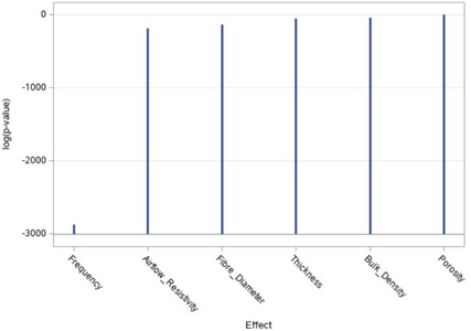
In Step 2, airflow resistivity entered the model. At this point, the selection method checks whether the first predictor, frequency, has become non-significant and if so, removes it. Frequency remained significant as expected since the sound absorption of a material is highly dependent on the frequency. The stepwise selection summary, Table 6, contains each variable that was added at each step of the process.
Table 6Stepwise model selection for sound absorption coefficient model
Step | Effect entered | Number effects in | F value | Pr > F |
0 | Intercept | 1 | 0.00 | 1.0000 |
1 | Frequency | 2 | 11607.3 | <.0001 |
2 | Airflow_Resistivity | 3 | 1758.12 | <.0001 |
3 | Thickness | 4 | 460.11 | <.0001 |
4 | Fibre_Diameter | 5 | 27.40 | <.0001 |
5 | Bulk_Density | 6 | 68.85 | <.0001 |
As can be seen from Table 6, porosity is missing. Porosity was shown to be not statistically significant and therefore removed as a possible predictor. Next, the Coefficient Progression for the sound absorption coefficient is determined which is illustrated in Fig. 5.
Fig. 5Selection fit criteria for sound absorption coefficient model
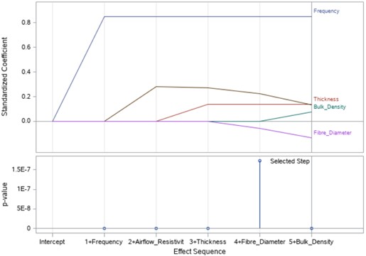
Fig. 5 shows the effect each variable has on the model and how the model changes as new variables are entered. Furthermore, it can be seen that at the start of the analysis, the airflow resistivity (dark brown line) had a significant effect but as the analysis progressed and more variables are added the overall effect airflow resistivity had on the model decreased.
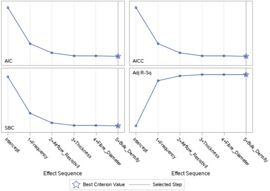
Thereafter, the set of fit criteria, AIC, SBC, AICC, and adjusted R-square values for each step are plotted and compared side-by-side as can be seen in Fig. 6. A model containing frequency, airflow resistivity, thickness, fibre diameter and bulk density, as predictors, is predicted by all model selection fit criteria, AIC, AICC, SBC, and the adjusted R-square value to be the best.
Fig. 6Selection fit criteria for sound absorption coefficient model
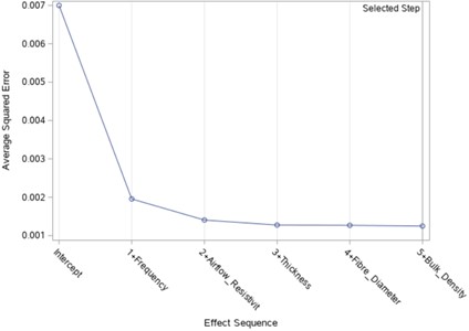
The Average Squared Error (ASE) is then calculated and plotted as illustrated in Fig. 7.
It can be seen from Fig. 7, that the ASE levels out after thickness is added to the model. Furthermore, the addition of the fibre diameter and bulk density decreases the ASE very little, this is most likely since airflow resistivity is highly dependent on these two variables.
Furthermore, several information criteria tests i.e., AIC, AICC, BIC, and SBC, were also conducted. All, the criteria tests uniformly agreed with the results obtained from the p-value criterion selection test, this is to say that AIC, AICC, BIC, and SBC ranked the model containing frequency, airflow resistivity, thickness, fibre diameter and bulk density as the best. The results for all the information criterion selection tests are not displayed for sake of brevity.
Fig. 7Progression of average squared error for sound absorption coefficient model
3.4. Sound absorption coefficient model selection
The model selection process requires applying the data to each model and analysing which model gives the highest adjusted R-squared value. During this process, every possible combination of the variables was checked to see which combination would give the highest adjusted R-squared value for the dataset, Microsoft Excel was utilized to perform this. The result of this process is expressed in Tables 7, 8.
Table 7Sound absorption coefficient model R-squared comparison
Combinations | F, AR, FD, BD, T (R2) | F, FD, BD, T (R2) | F, AR, FD, T (R2) | F, AR, BD, T (R2) | F, AR, FD, BD (R2) | F, T, AR (R2) | F, FD, BD (R2) | F, FD, AR (R2) | F, FD, T (R2) | F, BD, AR (R2) | F, BD, T (R2) |
Model type | |||||||||||
Log-log | 0.849 | 0.849 | 0.848 | 0.848 | 0.835 | 0.847 | 0.835 | 0.834 | 0.834 | 0.834 | 0.826 |
Exponential | 0.792 | 0.792 | 0.791 | 0.789 | 0.779 | 0.789 | 0.778 | 0.778 | 0.789 | 0.777 | 0.768 |
First-order polynomial with two-Interactions | – | – | – | – | – | 0.913 | 0.886 | 0.888 | 0.881 | 0.886 | 0.798 |
Third-order polynomial with three-interactions | – | – | – | – | – | 0.931 | 0.902 | 0.908 | 0.897 | 0.904 | 0.815 |
Footnote: F – frequency, AR - airflow resistivity, FD – fibre diameter, BD – bulk density, T – thickness | |||||||||||
Table 8Sound absorption coefficient model R-squared comparison
Combinations | F, AR, (R2) | F, FD (R2) | F, T (R2) | F, BD (R2) |
Model type | ||||
Log-log | 0.834 | 0.83 | 0.823 | 0.812 |
Exponential | 0.777 | 0.775 | 0.766 | 0.755 |
First-order polynomial with one-interaction | 0.884 | 0.84 | 0.757 | 0.761 |
Second-order polynomial with interactions | 0.901 | 0.856 | 0.773 | 0.777 |
From Table 7, it can be seen that the 3rd order polynomial with three interactions model gives the highest R-squared value. An interesting point to note is that this model is only dependent on frequency, airflow resistivity and thickness. This model has ten terms, however, despite the large number of terms, this model is surprisingly still simpler than current models. The final model will be selected later since further analysis for determining the best model is still necessary.
3.5. Sound absorption coefficient model comparison
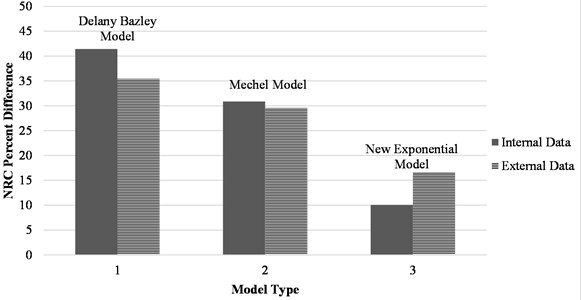
Fig. 8 displays the percentage difference between the measured and predicted sound absorption coefficient models developed in this research. Note, two validation datasets were used in this research, an internal dataset which was a subset taken from the main dataset and an external dataset which was compiled using literature data. The data for Fig. 8, was obtained by running the validation dataset in Table 9 through each model and then calculating the percentage difference between the NRC measured value and the NRC predicted value. The NRC was used since it is an average sound absorption coefficient value thus making it possible to compare the performance of each model.
Table 9Validation dataset
Sample No. | Thickness (mm) | Bulk density (kg/m3) | Porosity | Airflow resistivity (Pa.s/m2) | NRC |
Y23 | 12 | 31.78 | 10821.00 | 19.4 | 0.18 |
Y62 | 12.1 | 21.89 | 7190.71 | 19.4 | 0.14 |
R74 | 13 | 36.55 | 7878.88 | 29.7 | 0.15 |
R56 | 10.7 | 43.68 | 9183.22 | 29.7 | 0.15 |
G7 | 13.8 | 32.14 | 3846.84 | 40.8 | 0.14 |
G64 | 13.4 | 47.45 | 5205.24 | 40.8 | 0.15 |
B18 | 12.4 | 50.81 | 4129.30 | 49.5 | 0.13 |
B4 | 9.6 | 51.37 | 4142.01 | 49.5 | 0.14 |
B2 | 17 | 44.25 | 3114.57 | 49.5 | 0.17 |
B7 | 6.9 | 53.39 | 4782.71 | 49.5 | 0.10 |
G14 | 9.7 | 31.67 | 3402.13 | 40.8 | 0.11 |
G17 | 10.2 | 38.43 | 4093.42 | 40.8 | 0.13 |
G19 | 9.1 | 31.82 | 2871.38 | 40.8 | 0.11 |
G21 | 8.4 | 38.25 | 3691.78 | 40.8 | 0.13 |
G22 | 8.9 | 38.35 | 4087.86 | 40.8 | 0.14 |
G71 | 9.8 | 32.79 | 4026.94 | 40.8 | 0.13 |
R2 | 10.2 | 44.20 | 8665.41 | 29.7 | 0.16 |
R24 | 9.2 | 50.54 | 9283.67 | 29.7 | 0.17 |
R58 | 10.3 | 43.09 | 7760.59 | 29.7 | 0.15 |
R66 | 10.7 | 47.52 | 10828.33 | 29.7 | 0.16 |
R77 | 11.5 | 33.57 | 5820.87 | 29.7 | 0.14 |
Y22 | 9.5 | 31.72 | 11865.01 | 19.4 | 0.17 |
Y48 | 10.5 | 33.40 | 10806.63 | 19.4 | 0.18 |
From Fig. 8, it is evident that the exponential model overall attained the lowest percentage difference between the measured and predicted values for the internal and external datasets.
Fig. 8Sound absorption coefficient model comparison using internal and external data dataset
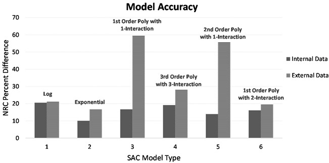
Table 10 evaluates all six sound absorption coefficient models that were developed. A selection metric has been developed as seen in Eq. (1). The selection metric attempts to give an objective value that can help identify the so-called “best” model:
where R2is the coefficient of determination, k is the number of predictors in the model and PD is the percentage difference between the measured value and the predicted value. It can be seen that the average Selection Metric for the exponential model is 1.58, which is 28.5 % higher than the next closest, which is the 1st order polynomial model. Hence, the Exponential model is selected as the best model.
Table 10Sound absorption coefficient best model selection
Model | R2 | Number of predictors (k) | Selection metric (SM) internal data | Selection metric (SM) external data |
Log | 0.849 | 4 | 1.03 | 1.00 |
Exponential | 0.792 | 4 | 1.97 | 1.19 |
1st Order Poly 1-Interaction | 0.884 | 3 | 1.76 | 0.50 |
3rd Order Poly 3-Interactions | 0.931 | 9 | 0.54 | 0.78 |
2nd Order Poly 1-Interaction | 0.901 | 5 | 1.29 | 0.32 |
1st Order Poly 2-Interactions | 0.913 | 6 | 0.95 | 0.37 |
3.6. Validating model assumptions
Before a model can be used for future predictions the model assumptions must be validated. The assumptions of linearity, independence, normality, and homogeneity of variances were all validated. Furthermore, the influential observations were tested and analysed. No influential data points were found when applying the Cook’s distance, using the software NumXL [13], in the dataset and hence no model adjustment was necessary.
Model linearity was validated using scatter plots of the response versus the predictor variables. The normality assumptions were validated by making use of a histogram plot of the residuals. The independence and equal variance assumptions were validated by making use of a residual plot of the errors.
4. Model derivation
The derivation of the model that has just been developed is now given. Linear regression analysis is used for the derivation of the developed models. Thereafter, the developed model is benchmarked against the currently existing models to evaluate its performance.
4.1. Derivation of sound absorption coefficient empirical equation
From the above analysis, it was shown that the variables frequency, airflow resistivity, thickness, bulk density, and fibre diameter are all statistically significant and therefore should be included in the sound absorption coefficient model. Therefore, the regression function in Microsoft Excel was utilized to do a regression analysis on the predictors selected. From the previous section, it was found that overall, the exponential model performed the best and hence was selected as the model of choice. Also, it must be noted that upon further analysis, it was found that including the airflow resistivity in the exponential model yielded no improvement and therefore was removed as a predictor. The derivation of the sound absorption coefficient regression model will now be carried out.
The exponential model to be derived is nonlinear and therefore needs to be transformed into a linear form. The nonlinear form of the equation is given in Eq. (2):
Simplifying the right side:
Then applying the law of logs:
ln(Y)=β0ln(e)+β1X1ln(e)+β2X2ln(e)+β3X3ln(e)+β4X4ln(e).
So that in the linear form:
Then substituting the independent variables that were selected i.e., frequency, fibre diameter, bulk density, and thickness, into Eq. (5), the formulation appears as follows:
Applying the natural log to the independent data in order to transform the data to a linear form is now applied. Since there is a lot of data an example only using data from one sample will be given.
Table 11Untransformed sound absorption coefficient data
Frequency (f) | Thickness (t) | Fibre diameter (df) | Bulk density (ρB) | Sound absorption coefficient (α) |
1000 | 9.5 | 40.8 | 47.83 | 0.111 |
Table 12Transformed sound absorption coefficient data
Natural log (ln) of: | ||||
Frequency (f) | Thickness (t) | Fibre diameter (df) | Bulk density (ρB) | Sound absorption coefficient (α) |
1000 | 9.5 | 40.8 | 47.83 | –2.198 |
Applying this transformation to the data and running a regression analysis in Microsoft Excel yields the regression model data illustrated in Table 13.
It can be seen from Table 13, that all variables are significant with p-values much less than the significance level criteria of αp= 0.05. Also, the adjusted R-squared value is 0.792, this is rather low, since using a 3rd order polynomial regression model to predict the sound absorption coefficient yields an R-squared value of 0.931 which is significantly higher. Nevertheless, it was shown in the previous section that the exponential model outperformed the 3rd order polynomial regression model when it came to prediction accuracy, hence the reason it was chosen. Now substituting the coefficients from Table 13 into Eq. (8), the following equation is derived:
Then transforming back to the nonlinear form, the following equation is arrived at:
where α is the sound absorption coefficient, f is the frequency in Hz, t is the material thickness in mm, df is the fibre diameter in μm, and ρB is the bulk density in kg/m3.
Table 13Microsoft excel regression statistics on sound absorption coefficient
Regression statistics | |||||
Multiple R | 0.889 | ||||
R square | 0.792 | ||||
Adjusted R square | 0.792 | ||||
Standard error | 0.337 | ||||
Observations | 4497 | ||||
ANOVA | |||||
df | SS | MS | F | Significance F | |
Regression | 4 | 1939.817 | 484.954 | 4268.736 | 0 |
Residual | 4492 | 510.318 | 0.114 | ||
Total | 4496 | 2450.136 | |||
Coefficients | Standard error | t Stat | P-value | ||
Intercept | –3.688 | 0.0409 | –90.088 | 0 | |
Frequency | 0.00109 | 8.59E-06 | 127.346 | 0 | |
Thickness | 0.0509 | 0.00299 | 17.0344 | 4.21E-63 | |
Fibre diameter | –0.00989 | 0.000443 | –22.351 | 5.2E-105 | |
Bulk density | 0.00437 | 0.000602 | 7.273 | 4.12E-13 | |
4.2. Model comparison using validation datasets
In this section, the model developed in this research is compared to the currently existing models using both the internal dataset and an external dataset. From this, the model performance is analysed.
Table 14 gives the model performance of the currently available sound absorption coefficient models for nonwoven fibrous materials. It can be seen that overall, the Mechel model performed best when compared to current models, with an average noise reduction coefficient percentage difference between the actual and predicted value of 30.86%. MatLab was used to perform all the calculations of the various models.
Table 14Sound absorption coefficient historical models comparison on internal dataset
Model | NRC minimum % difference | NRC maximum % difference | NRC average % difference |
Allard [5] | 19.85 | 79.23 | 46.38 |
Berardi [14] | 103.74 | 195.24 | 164.22 |
Delany & Bazley [3] | 15.82 | 57.63 | 41.43 |
Del Rey [15] | 203.66 | 293.66 | 232.15 |
Egab [16] | –643.53 | –394.10 | –480.38 |
Mechel [17] | 2.15 | 48.38 | 30.86 |
Miki [18] | 186.98 | 307.86 | 262.42 |
Garai [19] | 92.93 | 164.48 | 136.95 |
Komatsu [20] | 410.74 | 705.35 | 554.03 |
Liu [21] | 135.48 | 188.34 | 171.25 |
Ramis [22] | 108.45 | 333.35 | 160.03 |
Voronina [4] | 85.09 | 117.01 | 101.41 |
The average prediction error for the developed sound absorption coefficient exponential model compared with the two current best-performing models can be seen in Fig. 9. It is immediately evident that the developed sound absorption coefficient exponential model outperforms the currently available models on both datasets.
Fig. 9Viable model comparison on internal and external data
The literature data used to produce the external data graph in Fig. 9, was obtained from the following reference: Ballagh [23], Garai and Pompoli [19], Li et al. [24], Liy et al. [21], and Yang et al. [25].
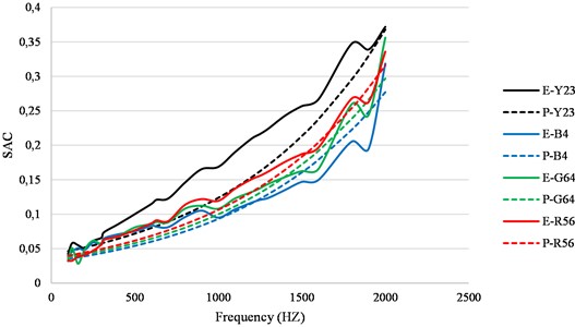
Fig. 10 visually demonstrates the prediction accuracy of the developed sound absorption coefficient exponential model on four different materials from the internal validation dataset. As can be seen, the exponential model closely follows the experimental data.
Fig. 10Prediction accuracy on validation dataset (solid lines represent experimental data and dotted lines represent model prediction)
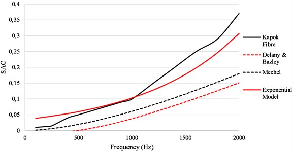
Furthermore, Figs. 11-12, demonstrates the prediction accuracy of the developed sound absorption coefficient exponential model against the currently existing best two models.
The experimental data plotted in Fig. 12, was obtained from reference [21]. The data was captured from a nonwoven specimen that was manufactured from 77 % kapok fibre and 23 % polypropylene fibre. The nonwoven had a thickness of 6 mm a bulk density of 45.07 kg/m3 and a mean fibre diameter of 17.9 μm. It must be noted that it is very difficult to find data in the literature with similar properties to the material that was developed in this research. This is simply because no regression models have been developed for this range of materials.
Thus, it can be seen from Figs. 11-12, that the sound absorption coefficient exponential model outperforms the current best models. Furthermore, the sound absorption coefficient exponential model also shows great flexibility in being able to accurately predict the sound absorption coefficient of a material that is made up of two different fibres, one being natural and the other being synthetic, as seen in Fig. 12.
Fig. 11Model accuracy comparison using internal data
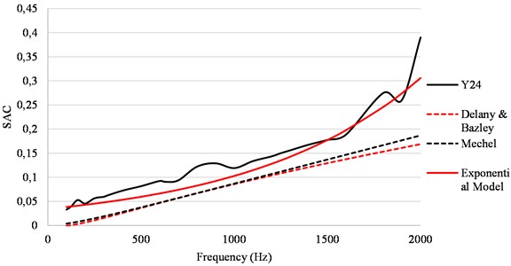
Fig. 12Model accuracy comparison using external data
5. Conclusions
From the onset of this research, the aim was to develop an empirical model that could accurately predicate the sound absorption coefficient of thin, low-density fibrous poroelastic materials in the low to mid-frequency range (100-2000 Hz). The reason is that currently, no existing empirical models can accurately predict in this range. Several empirical models were developed with the 3rd order polynomial regression attaining the highest adjusted R-squared value. Each developed model was then tested using a validation dataset, it was found that the exponential model outperformed the 3rd order polynomial regression model when it came to prediction accuracy on both the internal and external datasets. The reason for this may be that the 3rd order polynomial regression model was overfit to the data, thus giving the illusion that it was the “best” model due to the high adjusted R-squared value. Thereafter, the exponential model was benchmarked against the historic models in the literature, it was found to perform substantially better on both the internal dataset and external dataset. Furthermore, the exponential model showed great flexibility since it was able to accurately predict the sound absorption coefficient of a material that was made up of two different fibres. This also proves that the sound absorption coefficient model is adequate and can be used to predict the sound absorption coefficient for different types of materials within the range that the model was built for. Also, the sound absorption coefficient exponential model does not require airflow resistivity to be used for predictions, whereas almost all other current models require airflow resistivity. Thus, no experimental testing is required when using this model. This is a great advantage over the current models and will save the users time and resources. Therefore, it can be concluded that an exponential empirical model that can accurately predict the sound absorption coefficient of thin, low-density sound-absorbing materials was successfully developed using regression analysis.
References
-
M. Ayub, R. Zulkifli, M. H. Fouladi, N. Amin, and J. M. Nor, “A study on the acoustical absorption behavior of coir fiber using Miki model,” International Journal of Mechanical and Materials Engineering, Vol. 6, No. 3, pp. 343–349, 2011.
-
M. R. F. Kidner and C. H. Hansen., “A comparison and review of theories of the acoustics of porous materials,” International Journal of Acoustics and Vibration, Vol. 13, pp. 112–119, 2008.
-
M. E. Delany and E. N. Bazley, “Acoustical properties of fibrous absorbent materials,” Applied Acoustics, Vol. 3, No. 2, pp. 105–116, Apr. 1970, https://doi.org/10.1016/0003-682x(70)90031-9
-
N. Voronina, “Improved empirical model of sound propagation through a fibrous material,” Applied Acoustics, Vol. 48, No. 2, pp. 121–132, 1996.
-
J.-F. Allard and Y. Champoux, “New empirical equations for sound propagation in rigid frame fibrous materials,” The Journal of the Acoustical Society of America, Vol. 91, No. 6, pp. 3346–3353, Jun. 1992, https://doi.org/10.1121/1.402824
-
M. Kuhn and K. Johnson, Applied Predictive Modeling. New York, NY: Springer New York, 2013, p. 595, https://doi.org/10.1007/978-1-4614-6849-3
-
R. Dunne, D. Desai, and R. Sadiku, “A review of the factors that influence sound absorption and the available empirical models for fibrous materials,” Acoustics Australia, Vol. 45, No. 2, pp. 453–469, Jul. 2017, https://doi.org/10.1007/s40857-017-0097-4
-
A. Buchner et al., “G* Power 3.1 manual,” Heinrich-Heine-Universität: Düsseldorf, 2021.
-
D. C. Montgomery and G. C. Runger, Applied Statistics and Probability for Engineers. John Wiley & Sons, 2006.
-
K. Bellmann, “Fitting equations to data. Computer analysis of multifactor data,” Biometrische Zeitschrift, Vol. 17, No. 4, pp. 271–272, Jan. 2007, https://doi.org/10.1002/bimj.19750170415
-
D. C. Montgomery, E. A. Peck, and G. G. Vining, “Introduction to linear regression analysis,” in Probability and Statistics, Wiley, 2012, p. 679.
-
“Analytics Software and Solutions.”. https://www.sas.com/en_za/home.html
-
“NumXL – Analytics Made Easy!,” https://numxl.com/
-
U. Berardi and G. Iannace, “Predicting the sound absorption of natural materials: best-fit inverse laws for the acoustic impedance and the propagation constant,” Applied Acoustics, Vol. 115, pp. 131–138, Jan. 2017, https://doi.org/10.1016/j.apacoust.2016.08.012
-
R. D. Rey, J. Alba, J. P. Arenas, and V. J. Sanchis, “An empirical modelling of porous sound absorbing materials made of recycled foam,” Applied Acoustics, Vol. 73, No. 6-7, pp. 604–609, Jun. 2012, https://doi.org/10.1016/j.apacoust.2011.12.009
-
L. N. Egab, Xu Wang, S. K. B. Mazlan, and M. L. Choo, “Development of empirical models of polyfelt fibrous materials for acoustic application,” International Review of Mechanical Engineering (IREME), Vol. 7, No. 5, pp. 939–946, Jul. 2013, https://doi.org/10.15866/ireme.v7i5.3876
-
F. P. Mechel, “Expansion of the absorber formula by Delany and Bazley to low frequencies (in German),” (in German), Acustica, Vol. 35, pp. 210–213, 1976.
-
Y. Miki, “Acoustical properties of porous materials. Modifications of Delany-Bazley models.,” Journal of the Acoustical Society of Japan (E), Vol. 11, No. 1, pp. 19–24, Jan. 1990, https://doi.org/10.1250/ast.11.19
-
M. Garai and F. Pompoli, “A simple empirical model of polyester fibre materials for acoustical applications,” Applied Acoustics, Vol. 66, No. 12, pp. 1383–1398, Dec. 2005, https://doi.org/10.1016/j.apacoust.2005.04.008
-
T. Komatsu, “Improvement of the Delany-Bazley and Miki models for fibrous sound-absorbing materials,” Acoustical Science and Technology, Vol. 29, No. 2, pp. 121–129, Jan. 2008, https://doi.org/10.1250/ast.29.121
-
X. Liu, X. Yan, and H. Zhang, “Sound absorption model of kapok-based fiber nonwoven fabrics,” Textile Research Journal, Vol. 85, No. 9, pp. 969–979, Nov. 2014, https://doi.org/10.1177/0040517514557313
-
J. Ramis, R. Del Rey, J. Alba, L. Godinho, and J. Carbajo, “A model for acoustic absorbent materials derived from coconut fiber,” Materiales de Construcción, Vol. 64, No. 313, pp. e008–e008, Mar. 2014, https://doi.org/10.3989/mc.2014.00513
-
K. O. Ballagh, “Acoustical properties of wool,” Applied Acoustics, Vol. 48, No. 2, pp. 101–120, Jun. 1996, https://doi.org/10.1016/0003-682x(95)00042-8
-
L. Chengdong et al., “Material parameter determination in glass wool mat for sound absorption,” Applied Mechanics and Materials, Vol. 148-149, pp. 1271–1275, Dec. 2011, https://doi.org/10.4028/www.scientific.net/amm.148-149
-
T. Yang et al., “Study on the sound absorption behavior of multi-component polyester nonwovens: experimental and numerical methods,” Textile Research Journal, Vol. 89, No. 16, pp. 3342–3361, Nov. 2018, https://doi.org/10.1177/0040517518811940
About this article

No funding was provided for this research.
The datasets generated during and/or analyzed during the current study are available from the corresponding author on reasonable request.
Regan Dunne collected and analyzed the data, developed the sound absorption coefficient model, and wrote the paper. Dawood Desai and Stephan Heyns supervised the project and reviewed and edited the paper.
The authors declare that they have no conflict of interest.
