Abstract
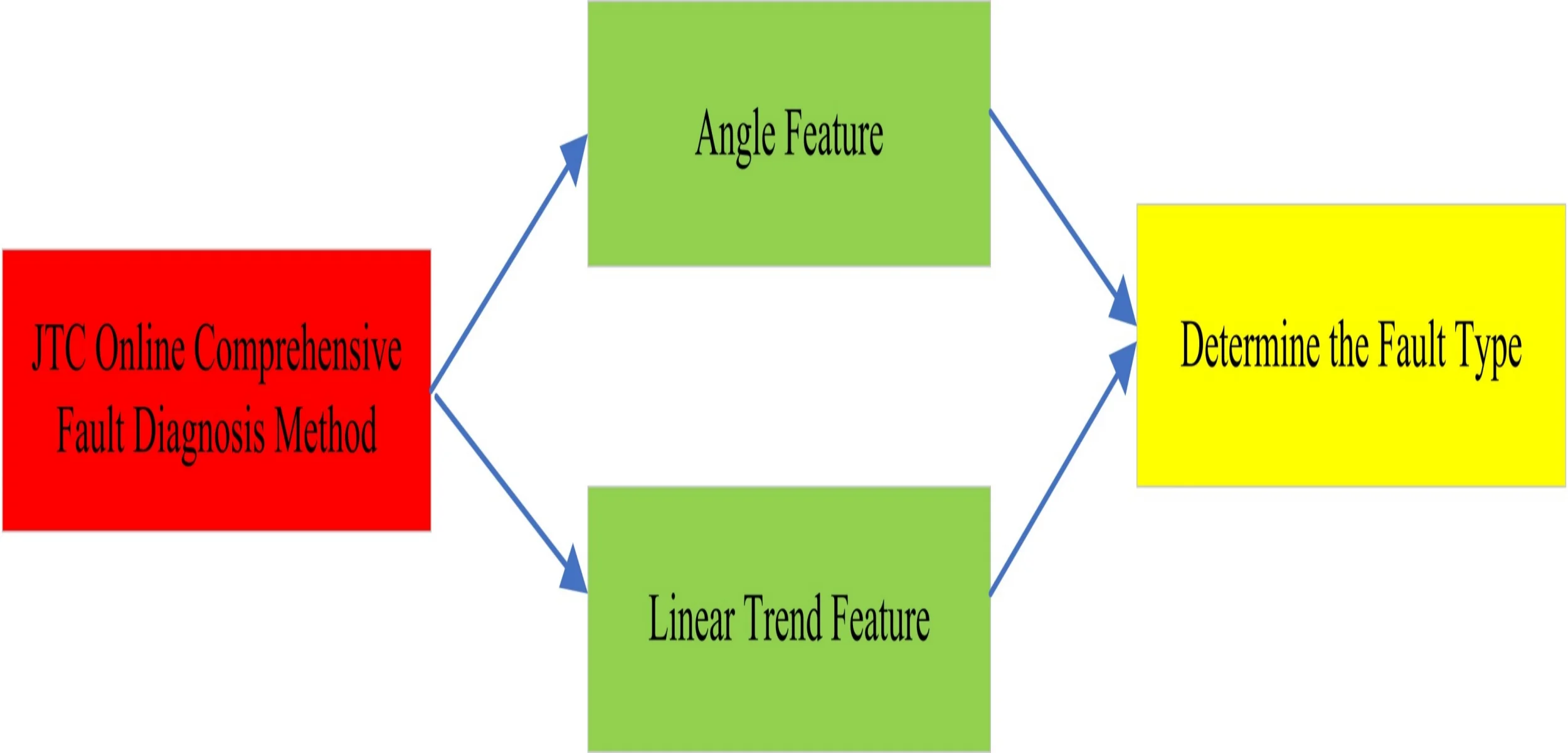
Aiming at the problem of incompatibility of the fault diagnosis method between JTC (Jointless Track Circuit) compensation capacitor and tuning zone, based on the amplitude envelope mathematical model of induced voltage of locomotive signal, an online comprehensive fault diagnosis algorithm for multi-compensation capacitor and tuning equipment fault was proposed. It is characterized by the angle of the tangent vector of the amplitude envelope at the compensation capacitor and the linear trend within the three compensation capacitor sections close to the transmitter when the tuning device fails, the angle feature and linear trend feature are extracted to determine the fault type. Experimental results show that the proposed algorithm can accurately detect multi-compensation capacitor faults and tuning equipment faults with high accuracy and high efficiency, especially the sudden multi-compensation capacitor faults and tuning zone unit breaking faults. The accuracy of the algorithm for JTC fault diagnosis is verified under different signal-to-noise ratio and ballast resistance fluctuation, which shows that the algorithm has strong applicability.
Highlights
- A new JTC online comprehensive fault diagnosis method is proposed.
- The problem of incompatibility of the fault diagnosis method between JTC compensation capacitor and tuning zone is solved.
- This method has strong adaptability to the fluctuation of ballast resistance in different signal-to-noise ratio and ballast resistance fluctuation, and has certain engineering feasibility.
- The detection data of this method are all from the track circuit, and the detection content is more comprehensive, which provides a reliable basis and a new idea for railway fault diagnosis.
1. Introduction
As an important part of train control system in China, JTC plays an important role in ensuring the safety and transportation efficiency, JTC mainly consists of the main track circuit and tuning zone. The main track circuit counteracts the high inductance of the rail by paralleling a certain amount of compensation capacitors at the upper interval of the rail, so that the rail presents a whole resistance. The electrical isolation was realized between adjacent track circuits through the resonant relationship between tuning units and the signal frequency in the tuning zone, in which include BA1 and BA2 and the hollow coil SVA [1]. Compensation capacitor failure will shorten the effective transmission distance of JTC and reduce the minimum shunt current, and even lead to the occurrence of track circuit red tape. Tuning equipment failure will cause cross-talk between signals in adjacent sections [2]. The failure of JTC compensation capacitor and tuning equipment will not only affect the normal transmission of signal, but even endanger the safety of driving. At present, regular inspection of compensation capacitor and tuning equipment is mainly carried out by electrical inspection vehicle, but there are problems of high detection cost and poor timeliness [3].
Existing researches mainly focus on fault diagnosis of compensation capacitor [4-14], simulated annealing algorithm and fast diagnosis algorithm of multiple compensation capacitor can realize combined fault diagnosis of compensation capacitor [14, 15], however, intelligent search algorithms such as simulated annealing algorithm take a long time to perform real-time diagnosis of track circuits. The multi-compensation capacitor fast diagnosis algorithm is suitable for the simultaneous failure of two or less compensation capacitors. The combination fault detection of multiple compensation capacitor can also be realized by using the knowledge of neural fuzzy system [16], deep learning and decision tree [17-19], considering the execution time of these intelligent algorithms is generally long, it is only suitable for off-line analysis of compensation capacitor. The above algorithms do not take the tuning zone fault into account, resulting in the application of these methods has great limitations [20], so that the comprehensive diagnosis of JTC fault cannot be realized. Improving the detection method of compensation capacitor is a very necessary and urgent work to do. Therefore, this paper proposed a real-time diagnosis algorithm of multi-compensation capacitor combined with tuning equipment to meet the actual needs of the railway site.
2. Related research work
2.1. Mathematical model of compensation capacitor and tuning region
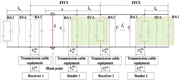
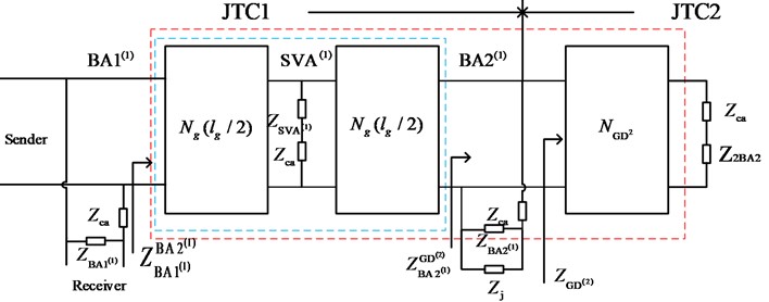
JTC is mainly composed of sending and receiving terminal equipment and rail lines in this section. The sending end part mainly refers to the tuning equipment and the cable equipment at the sending end and the transmitter; Similarly, the receiving end part mainly includes the tuning equipment at the receiving end, the receiving end cable equipment and the receiver; The rail line includes the rail between the sending end and the receiving end and the compensation capacitor in parallel at equal intervals. When the train runs in track section 1, the JTC under the shunt condition is shown in Fig. 1.
Fig. 1JTC shunt status structure diagram
Through analysis, the relationship between the shunt current and the shunt point is:
At this time, the induced voltage amplitude envelope signal recorded by the locomotive signal is:
where US(t) is the frequency shift signal output by transmitter 1, α=α1α2, α1 can be approximated as a constant, which is determined by the characteristic parameters the receiving coil and the frequency of JTC signal. α2 is a constant, which determined by the internal circuit of the locomotive signal. Rf is the shunt resistor, G(x) is the four-terminal network transmission matrix from the shunt point to sender 1, Tp is the transmission matrix of four-terminal network for the sending device, Tt is a four-terminal network transmission matrix for the sender tuning zone, Tg(x) is the four-terminal network transmission matrix of rail line from the train shunt point to the rail surface of the tuning-zone of the sending end.
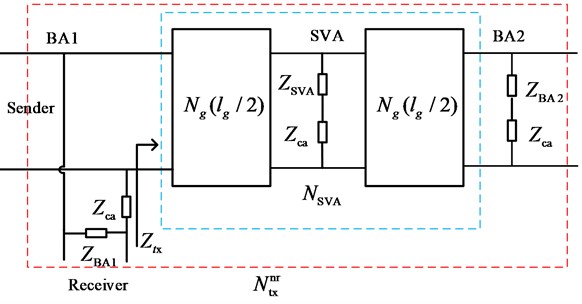
The tuning zone effectively isolated the signal transmission between adjacent track circuits through BA1, BA2 and SVA, which presented a series and parallel resonance relationship between the signals in this section. ZBA1, ZBA2 and ZSVA respectively represent the impedance values of BA1, BA2 and SVA at the frequency signals in this section; Zca represents the impedance value of each device when it is connected with the rail; Ng(lg/2)is the equivalent four-terminal network of half rail line length in the tuning zone; At this time, the four-terminal network model of the tuning zone is shown in Fig. 2, where NSVA is the equivalent four-terminal network matrix of the sum of the SVA equivalent impedance of the hollow coil ZSVA and the impedance of the rail connection Zca, then, the equivalent four-terminal network matrix between tuning unit BA1 and BA2 can be expressed as:
Ng(lg/2) is the equivalent four-terminal network matrix of half rail line length in the tuning zone:
NSVA is the equivalent four-terminal network matrix of hollow coil SVA:
Ztx is the apparent impedance from tuning region BA1 to BA2, expressed as:
When the tuning zone is fault-free, the equivalent four-terminal network matrix at the sending end is Nnrtx:
2.2. Compensation capacitor and tuning zone fault modeling and impact analysis
The compensation capacitor and BA1 and BA2 and SVA are connected to the rail through rail lead wiring, due to the complex operating environment and man-made damage, the compensation capacitor disconnection or the value of capacitor dropping or the fault of tuning zone will be caused.
Fig. 2JTC Tuning zone normal state four terminal network model
(ⅰ) When a line break fault occurs in BA1, its fault equivalent four-terminal network model can be treated the value of ZBA1 as infinity, that is, it can be simulated according to the disconnection state. The four-terminal network model of the tuning region under BA1 disconnection is shown in Fig. 3.
Fig. 3Four-terminal network model of tuning zone when BA1 fails
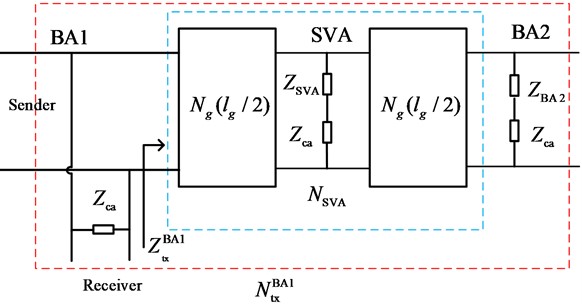
It can be obtained that the equivalent four-terminal network matrix of the tuning-zone of the sender under BA1 disconnection is NBA1tx:
(ⅱ) when BA2 breaks, its equivalent circuit model is shown in Fig. 4, where ZGD(2) is the apparent impedance from the tuning region at the receiving end of track circuit 1 to the sending end of track circuit 2:
ZGD(2)BA2(1) is the apparent impedance of track circuit 2:
ZBA2(2)BA1(1) is the apparent impedance from BA2 to track circuit 2:
therefore, the equivalent four-terminal network matrix of the tuning-zone of the sender in the case of l BA2 disconnection is:
(ⅲ) according to FIG. 2, the equivalent four-port network matrix of the tuning-zone at the sending end under SVA disconnection of the hollow coil is NSVAtx:
Fig. 4The equivalent circuit model when BA2 is fault
Eqs. (1-14) are used, according to the electrical parameters of the uninsulated track circuit, select a section of track circuit and simulate the states of fault free, compensation capacitor disconnection and tuning equipment fault respectively. The corresponding simulation conditions: the carrier signal frequency of track circuit 1 is f1=2000 Hz and 2 is f2=2600 Hz. The length of track circuit 1 is lg1=1099 m and 2 is lg2=1442 m. The number of compensation capacitors are nc1=11 and nc2=18, the value of cv1=40 μF and cv2=50 μF, the shunt resistance is Rf=0.15 Ω, the ballast resistance is RG= 1 Ω·km, The result is shown in Fig. 5.
As can be seen from Fig. 5, when the track circuit is not equipped with compensation capacitor, I(x) is the normalized shunt current and will attenuate greatly from the sending end to the receiving end.
As can be seen from Fig. 6, the track circuit equipped with compensation capacitor make the shunt current present a “wave” rise from the receiving end to the sending end of the local section under the condition of no fault. When the compensation capacitor breaks the line, I(x) will attenuate rapidly at the breakpoint, making the angle between the left and right side tangents of the breakpoint curve increased to 180 degrees.
Fig. 5Normalized of all compensation capacitor failures
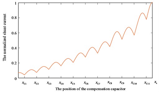
Fig. 6Normalized of fault-free and C5, C9 disconnection
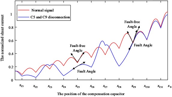
Fig. 7Normalized I(x) of fault-free and tuning device failure
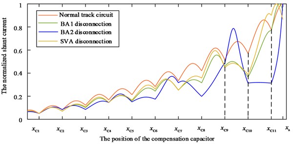
As can be obtained from Fig. 7, when the tuning equipment fails, the overall trend between the three compensation capacitors near the sending end will change.
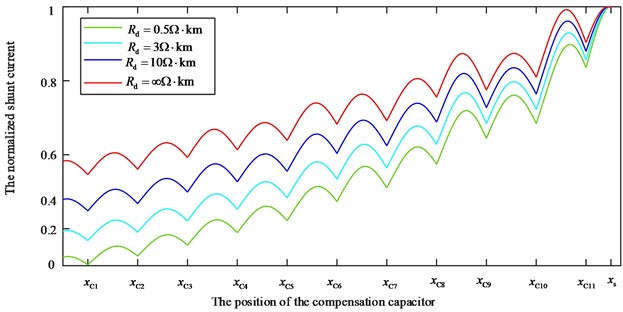
As shown in Fig. 8, the fluctuation of ballast resistance will affect the attenuation rate of I(x). The larger the resistance is, the smaller the attenuation rate will be, and the greater the vice versa. However, the change of ballast resistance will not change the overall trend of the curve and the tangent angle at the position of compensation capacitor.
Fig. 8Normalized I(x) of fluctuation on ballast resistor
3. Methodology
3.1. Angle feature extraction
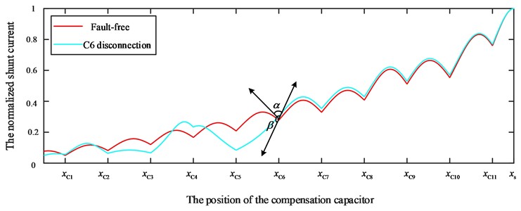
According to Fig. 9 and the above analysis, when line breaking occurs on the compensation capacitor C6, the included angle of the tangent vector on the left and right sides of C6 increases from α to β. Therefore, the included angle of the tangent vector on the left and right sides of the compensation capacitor is used as the basis for fault feature extraction. In order to obtain the tangent vectors of the left and right sides of the compensation capacitor, the curve equations of both sides should be obtained respectively. According to the data set I(x) obtained by simulation, the data {(xl,yl),l=0,1,2,⋯,t} at the distance of t between the two sides of the compensation capacitor and its position is selected for polynomial fitting:
where m is the number of compensation capacitor. Then we can see from the above formula that 2m curves need to be fitted. Set the fitting model be:
Fig. 9Tangent vector angle extraction diagram for C6 normal and C6 disconnection
The least square method was used to determine the coefficients of a0,a1,⋯an, assuming the weight of each data point is 1, φ(a0,a1,⋯,an) is minimized, that is minimizing:
then there is:
where j=0,1,2,⋯,t, thus:
According to Eqs. (15)-(17), the equations can be obtained as follows by solving Eq. (18):
This equation is called the normal equation of polynomial fitting.
By setting:
There is XA=Y, thus A=X-1Y, Eq. (17) can be obtained by solving the coefficient vector A from the matrix equation. The left and right side tangent vectors of the fitting polynomial at xi arev1=(1,d(S-(xi))dxi) and v2=(1,d(S+(xi))dxi), the angle between the left and right side tangent vectors of theta is θi=arccosv1⋅v2‖v1‖⋅‖v2‖, define the fault angle determination indicator as Ji=1+cosθi2, (0≤Ji<1).
According to the above analysis and a large number of railway field data, the more serious the reduction of compensation capacitor, the larger the angle of tangent vector θ, the smaller the angle determination index Ji, and when the compensation capacitor is broken, Ji is 0.
3.2. Piecewise linear feature extraction
According to the I(x) simulation curve of tuning equipment fault, the fault characteristics occur in the first three compensation capacitor segments close to the sending end. Therefore. I(x) is divided by the location of the first three compensation capacitors close to the sending end, that is to say:
where k=1,⋯,4, lk(m-2)(xm-2), lk(m-2)(xm-2), l(m-2)(xm-2) refers to the segments sequentially captured at the first three the position of compensation capacitor near the sending end respectively, and linear fitting is carried out on them:
Eq. (22) represents the linear segment obtained by connecting the shunt current at the compensation capacitor. According to Eq. (22), the overall trend of divided fragments Qk=[qk(m-2),qk(m-1),qkm] can be extracted as follows:
According to Eq. (21)-(23), JTC without fault, BA1 broken line, BA2 broken line and SVA broken line were simulated respectively and the overall trend of segment division was extracted, that is Q1=[1,1,1], Q2=[0,1,1], Q3=[0,0,1], Q4=[0,1,0].
3.3. Fault mode diagnosis method
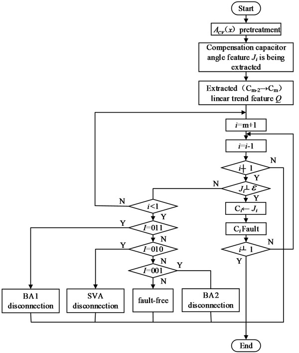
The fault diagnosis process is shown in Fig. 10. The pre-processing of I(x) includes signal coordinate transformation and amplitude normalization. The signal coordinate transformation adopts spline interpolation method, and the position of compensation capacitor is taken as I(x) transformed horizontal coordinate to eliminate the influence of train speed change. The angle feature and the linear trend feature vector of I(x) of the tuning region are first extracted based on the JTC fault feature extraction method proposed in this paper. Then from the sending end, the angle feature Ji of all compensation capacitor are tested to test if they are less than or equal to the decision threshold ε. If the conditions are met, the fault Ci will be output and the linear trend feature vectors of the tuned devices will not be tested. If the detection results show that all values Ji are greater than the decision threshold ε, it means that no line breaking fault occurs in the compensation capacitor, and the tuning device is detected according to the extracted linear characteristic trend vector Q of the tuning device. Finally, the test result is output.
4. Algorithm evaluation criteria and parameter determination
Suppose that the total number of diagnosed JTC is ws, the number of sections determined by the algorithm to be faulty capacitors or faulty tuning devices and detected to be normal capacitors or normal tuning devices is wf, the number of segments that the algorithm determines to be normal capacitors or normal tuning devices and the electrical detection vehicle detects to be faulty capacitors or faulty tuning devices is wm, the number of areas where the fault is detected by the algorithm and the electrical detection vehicle, but the detection results are inconsistent is wu. By the above definition, the false negative rate is hl, the false positive rate is hw, the false alarm rate hx and the accuracy rate is hz, where:
Fig. 10Fault diagnosis flowchart of compensation capacitor and tuning device
Eq. (24) is used to represent the probability that the compensation capacitor or tuning device fault exists in the segment and is diagnosed as normal by the proposed algorithm:
Eq. (25) is used to represent the probability that the compensation capacitor or tuning device fault occurs in the segment and is diagnosed as other faults by the proposed algorithm:
Eq. (26) is used to represent the probability that the segment is fault-free and the proposed algorithm diagnoses the fault of compensation capacitor or tuned equipment:
Eq. (27) is used to represent the probability that the diagnosis result of the algorithm in this paper is consistent with the section fault condition.
Based on the evaluation indexes defined above, JTC with the number of compensation capacitor ranging from 7 to 16 is selected for simulation analysis. When the tolerance value drops to the compensation capacitor, the angle between the left and right side tangent vectors of I(x) is greater than 168 degrees, it is considered that the compensation capacitor has broken line fault. Through a large number of simulation analysis, when the distance t between the two sides of the compensation capacitor is 9, the degree of fitting polynomial n is 3, and the decision threshold ε is 0.01, an optimal balance can be reached for hlhwhx and hz.
5. Experiments
5.1. Simulation experiment verification
The fault diagnosis algorithm proposed in this paper is used to diagnose the faults in the normal state of JTC and when C4 and C7 are disconnected. The corresponding simulation parameters are set as follows: signal-to-noise ratio SNR=50 dB, ballast resistance RG=1 Ω⋅km.
According to the fault diagnosis flow chart shown in Fig. 10, the detection result of compensation capacitor of a certain line electrical detection vehicle is diagnosed, and the detection result is shown in Fig. 11.
Fig. 11I(x) with noise of fault-free and C4, C7 disconnection
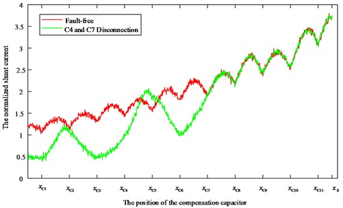
Fig. 12Angle feature vector extraction result of fault-free and C4, C7 disconnection
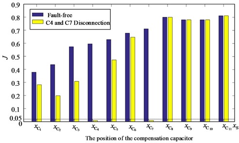
The extracted angle feature extraction results are shown in Fig. 12, the angle feature at the position of C4 and C7 in the figure are less than the decision threshold, and the diagnostic results show that C4 and C7 have line breaking faults.
According to the fault diagnosis flow chart shown in Fig. 10, the detection result of compensation capacitor of a certain line electrical detection vehicle is diagnosed, and the detection result is shown in Fig. 13.
Fig. 13Ixwith noise of fault-free and BA1 disconnection
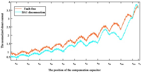
Fig. 14Angle feature extraction results of fault free and BA1 disconnection
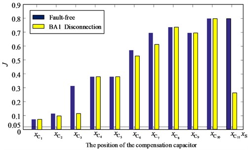
Fig. 15Linear trend feature extraction results of fault-free and BA1 disconnection
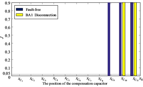
The extraction result of Angle feature in Fig. 14 shows that the compensation capacitor does not fail in Fig. 13, and the linear trend feature is extracted, the extraction result is Q=[0,1,1], as shown in Fig. 15, indicating that BA1 disconnection.
Similarly, the broken line of BA2 was simulated respectively and the overall trend of this section was extracted.
As shown in Fig. 16, the extraction result is Q3=[0,0,1] it means that BA2 has broken the line.
The situation of SVA disconnection was simulated respectively and the overall trend of this section was extracted.
Fig. 16Linear trend feature extraction results of fault-free and BA2 disconnection
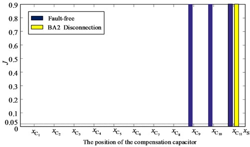
Fig. 17Linear trend feature extraction results of fault-free and SVA disconnection
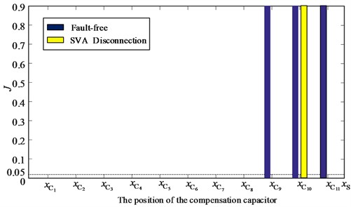
As shown in Fig. 16, the extraction result is Q3=[0,1,0] it means that BA2 has broken the line.
The above experiments show that the algorithm has accurate detection effect on multiple compensation capacitor disconnection and tuning equipment breaks.
5.2. Algorithm performance analysis
In order to verify the accuracy of the proposed method in JTC fault diagnosis under different signal-to-noise ratio and ballast resistance fluctuation, according to the above simulation model and the track circuit adjustment table, the signal-to-noise ratio SNR is 30 dB, 40 dB, 50 dB and 60 dB respectively, and the resistance of ballast is 0.5 Ω·km, 1 Ω·km, 3 Ω·km and 5 Ω·km respectively. 100 Ω·km, ∞ Ω·km, selected 69 groups of sample data corresponding to various fault modes (tuning equipment fault, compensation capacitor combination fault) of each parameter, and obtain a total of 1656 groups of sample data including various fault modes. Finally, obtained hlhwhx and hz under different signal-to-noise ratio and different ballast resistance, as shown in Table 1 and Table 2.
As can be seen from Table 1 and Table 2, the larger the signal-to-noise ratio SNR is, the larger the value of hz is, and the value of hl, hw, and hx also changes to a very small value, and the higher the diagnosis accuracy is. When the SNR is small, the fitting accuracy will be affected, and the extracted angle features will be inaccurate, thus affecting the accuracy of fault diagnosis. The change of ballast resistance has no effect on the fitting accuracy, and the fluctuation of ballast resistance basically does not affect the fault diagnosis rate. When the SNR exceeds 50 dB, no matter how the ballast resistance changes, the diagnosis accuracy exceeds 94.2 %; This method is simpler than deep learning algorithms and decision tree algorithms, and has higher diagnosis accuracy than BP neural network algorithms, and has better flexibility and applicability.
Table 1Algorithm performance simulation test results Eq. (1)
SNR (%) | RG | |||||||||||
0.5 Ω·km | 1 Ω·km | 3 Ω·km | ||||||||||
hz | hx | hl | hw | hz | hx | hl | hw | hz | hx | hl | hw | |
30 dB | 81.2 | 11.6 | 4.3 | 2.9 | 82.6 | 13.0 | 1.4 | 2.9 | 81.2 | 13.0 | 4.3 | 2.9 |
40 dB | 89.9 | 7.2 | 1.4 | 1.4 | 92.8 | 7.2 | 0 | 0 | 95.7 | 2.9 | 1.4 | 0 |
50 dB | 94.2 | 4.3 | 1.4 | 0 | 97.1 | 1.4 | 0 | 1.4 | 98.6 | 1.4 | 0 | 0 |
60 dB | 95.7 | 4.3 | 0 | 0 | 97.1 | 1.4 | 0 | 0 | 97.1 | 2.9 | 0 | 0 |
Table 2Algorithm performance simulation test results Eq. (2)
SNR (%) | RG | |||||||||||
10 Ω·km | 100 Ω·km | ∞ Ω·km | ||||||||||
hz | hx | hl | hw | hz | hx | hl | hw | hz | hx | hl | hw | |
30 dB | 82.6 | 11.6 | 1.4 | 2.9 | 81.2 | 11.6 | 5.8 | 1.4 | 85.5 | 10.1 | 1.4 | 2.9 |
40 dB | 94.2 | 15.8 | 0 | 0 | 95.7 | 2.9 | 1.4 | 0 | 94.2 | 2.9 | 0 | 2.9 |
50 dB | 98.6 | 11.4 | 0 | 0 | 97.1 | 2.9 | 0 | 0 | 98.6 | 1.4 | 0 | 0 |
60 dB | 98.6 | 0 | 0 | 1.4 | 97.1 | 2.9 | 0 | 0 | 98.6 | 1.4 | 0 | 0 |
6. Conclusions
In order to solve the problem that the fault detection methods of JTC compensation capacitor and tuning region are incompatible, an online comprehensive fault diagnosis algorithm is proposed to solve the fault of multiple compensation capacitor and tuning equipment. The experimental results show that the proposed algorithm has a high diagnosis accuracy in the case of large SNR, and the diagnosis results are basically not affected by the fluctuation of ballast resistance, so that the comprehensive fault diagnosis of JTC is well realized. It can accurately detect the combined fault of multiple compensation capacitors, and can also quickly and accurately detect the fault of tuning equipment without superimposed compensation capacitor fault. In particular, the sudden multi-compensation capacitor fault and the unit disconnection fault in the tuning region overcome the disadvantage that the previous method can only diagnose the local fault of JTC. In the case of different signal-to-noise ratio and ballast resistance fluctuation, this detection method has a strong adaptability for the fluctuation of ballast resistance and certain engineering feasibility.
References
-
W. Dong, “Fault diagnosis for compensating capacitors of jointless track circuit based on dynamic time warping,” Mathematical Problems in Engineering, Vol. 2014, pp. 1–13, Jan. 2014, https://doi.org/10.1155/2014/324743
-
L. H. Zhao and L. Ren, “Study on influence of JTC adjacent section interference on TCR,” Journal of the China Railway Society, Vol. 35, No. 12, pp. 52–56, 2013.
-
S. P. Sun and H. B. Zhao, “The method of fault detection of compensation capacitor in jointless track circuit based on phase space reconstruction,” Journal of the China Railway Society, Vol. 34, No. 10, pp. 79–84, 2012.
-
L. H. Zhao et al., “A comprehensive fault diagnosis method for jointless track circuit based on genetic algorithm,” Journal of the China Railway Science, Vol. 31, No. 3, pp. 107–113, 2010.
-
L. H. Zhao et al., “Compensation capacitor fault detection in jointless track circuit based on Levenberg-Marquard algorithm and generalized s-transform,” Control Theory and Application, Vol. 27, No. 12, pp. 1663–1668, 2010.
-
L. H. Zhao and J. C. Mu, “Fault diagnosis method for jointless track circuit based on AOK-TFR,” Journal of Southwest Jiaotong University, Vol. 46, No. 1, pp. 84–91, 2011.
-
L. H. Zhao, B. G. Cai, and K. M. Qiu, “The method of diagnosis of compensation capacitor failures with jointless track circuits based on HHT and DBWT,” Journal of the China Railway Society, Vol. 33, No. 3, pp. 49–54, 2011.
-
L. H. Zhao et al., “Fault diagnosis system for compensation capacitors of jointless track circuit based on layered immune mechanism,” Journal of the China Railway Society, Vol. 35, No. 10, pp. 73–81, 2013.
-
S. P. Sun et al., “Equipment fault diagnosis for electrical separation joint of jointless track circuits using qualitative trend analysis,” Journal of the China Railway Society, Vol. 35, No. 1, pp. 105–113, 2014.
-
L.-H. Zhao, C.-L. Zhang, K.-M. Qiu, and Q.-L. Li, “A fault diagnosis method for the tuning area of jointless track circuits based on a neural network,” Proceedings of the Institution of Mechanical Engineers, Part F: Journal of Rail and Rapid Transit, Vol. 227, No. 4, pp. 333–343, Mar. 2013, https://doi.org/10.1177/0954409713480453
-
L. Oukhellou, A. Debiolles, T. Denœux, and P. Aknin, “Fault diagnosis in railway track circuits using Dempster-Shafer classifier fusion,” Engineering Applications of Artificial Intelligence, Vol. 23, No. 1, pp. 117–128, Feb. 2010, https://doi.org/10.1016/j.engappai.2009.06.005
-
L. Zhao, Y. Maggie Guo, and B. D. Klein, “Analysis of structure importance of compensation capacitor in jointless track circuit,” Proceedings of the Institution of Mechanical Engineers, Part F: Journal of Rail and Rapid Transit, Vol. 231, No. 3, pp. 329–344, Nov. 2016, https://doi.org/10.1177/0954409716630338
-
Y. B. Cui et al., “Fault diagnosis method for JTC rail surface equipment based on stock analysis and grey correlation analysis,” Journal of the China Railway Society, Vol. 43, No. 5, pp. 112–120, 2021.
-
K. Xu and L. Zhao, “A rapid diagnosis method for multiple compensation capacitor faults of jointless track circuits,” Journal of the China Railway Society, Vol. 40, No. 2, pp. 67–72, 2018, https://doi.org/10.3969/j.issn.1001-8360.2018.02.010
-
Y. P. Zhang et al., “A comprehensive fault detection method for jointless track circuit based on SA algorithm,” Journal of the China Railway Society, Vol. 39, No. 4, pp. 68–72, 2017.
-
J. Chen, C. Roberts, and P. Weston, “Fault detection and diagnosis for railway track circuits using neuro-fuzzy systems,” Control Engineering Practice, Vol. 16, No. 5, pp. 585–596, May 2008, https://doi.org/10.1016/j.conengprac.2007.06.007
-
Z. Y. Zheng et al., “Research on fault detection for ZPW-2000A jointless track circuit based on deep belief network optimized by improved particle swarm optimization algorithm,” IEEE Access, Vol. 8, pp. 175981–175997, 2020.
-
X. X. Xie and S. H. Dai, “Fault diagnosis of jointless track circuit based on deep learning,” Journal of the China Railway Society, Vol. 42, No. 6, pp. 79–85, 2020.
-
W. B. Zhu and X. M. Wang, “Research on fault diagnosis of railway jointless track circuit based on combinatorial decision tree,” Journal of the China Railway Society, Vol. 40, No. 7, pp. 74–79, 2020.
-
Y. P. Zhang and T. W. Zhu, “Comprehensive fault diagnosis method for jointless track circuit based on fuzzy qualitative trend analysis,” Journal of Chongqing University, Vol. 42, No. 3, pp. 65–75, 2019.
About this article

The authors have not disclosed any funding.
The datasets generated during and/or analyzed during the current study are available from the corresponding author on reasonable request.
Ming Zhu provided all the railway field test data. Qiang Zhang and Taowei Zhu completed the methodology and the simulation experiment. Qiang Zhang wrote the entire research paper.
The authors declare that they have no conflict of interest.
