Research on residual useful life prediction of li-ion battery based on GA-LM-BPNN

1. Introduction

The prediction of Li-ion battery is the focus of the whole residual useful life (RUL) prediction [1]. Dong proposed a sub-optimal method for health diagnosis of satellite Li-ion batteries based on Auto Vector Regression and Particle Filter (AVR-PF) [2]. In order to overcome the problems of high dependence model and poor adaptability of single prediction method, Back Proragation Neural Network (BPNN) was improved, and the fusion data-driven method was adopted to predict the RUL of Li-ion battery [3].

2. Test conduct and analysis of li-ion battery

The charging and discharging process of lithium-ion batteries is the same as the process of completing the corresponding energy conversion. In the production process of Li-ion batteries, irreversible chemical reactions occur inside the batteries, resulting in the electrode loss and increasing internal resistance [4-5]. These changes in internal resistance are the main parameters corresponding to the degradation. An important step is to establish its life degradation model. However, it is not easy to establish the ideal model of battery degradation accurately in practical application. Based on a large number of experimental data, NASA’s PCoE research center proposed a simple and feasible battery equivalent model to predict the RUL. The equivalent model is shown in Fig. 1.

Fig. 1Equivalent model

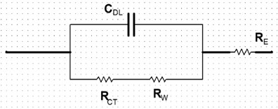
Where, $C_{DL}$ is the double-layer capacitance; $R_{CT}$ is the transfer resistance; $R_W$ is the Warburg impedance, and $R_E$ is the electrolyte resistance. After analyzing the data, NASA researchers found that the effect of $R_W$ and $C_{DL}$ on the life degradation is negligible, but has a high linear relationship with $R_{CT}+R_E$. They verified a high linear correlation between the capacity and impedance parameters of Li-ion batteries, as shown in Fig. 2. Saha et al. proposed the following empirical model to describe Li-ion batteries [6]:

where, $C_k$ is the capacity in the $k$ cycles; $\mathrm{\Delta }{t}_k$ is the rest time between two adjacent charging and discharging cycles; ${\beta }_1$ and ${\beta }_2$ is a specific parameter of the battery empirical model. ${\eta }_C$ is the coulomb efficiency, which is used to express the percentage between the total amount of charge released by the battery and the total amount of charge charged. In Li-ion batteries, increasing the rest time after charging and discharging can increase the capacity in the next cycles.

It is not difficult to see from the above analysis that the capacity will gradually decrease with the aging of Li-ion battery. The capacity charging is basically gradually away from the nominal capacity, so it can be used to predict the RUL of capacity.

In this paper, the test data of capacity to be used is 1.1 Ah. The whole experiment data is mainly composed of the discharge of the charging part and the battery capacity. The charging experimental data includes impedance data, charging voltage and charging current data. The discharge experimental data includes impedance data, discharge voltage and discharge current data, as well as the corresponding ambient temperature test time and other information. The experimental process can be described as follows.

(1) The ambient temperature of the experiment is 20 ℃-25 ℃;

(2) Charging mode: the constant current is 0.675 A and the maximum voltage is 4.2 V;

(3) Discharge mode: the constant current is 1.35 A, the minimum voltage is 2.7 V, and the discharge rate is 1C;

(4) Electrochemical impedance spectroscopy was used for measurement;

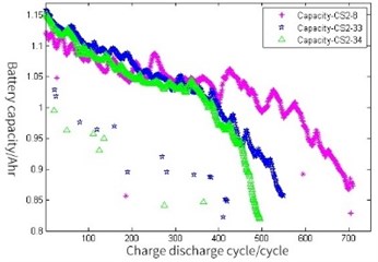
(5) Select the Capacity-CS2-8#, Capacity-CS2-33#, Capacity-CS2-34#of Battery Data Set as the experimental data. The degradation curve is shown in Fig. 3. When the battery capacity reaches 80 % of the nominal capacity, the experiment will be stopped. Because the nominal capacity is 1.1 Ah, and the capacity threshold is 0.88 Ah.

Fig. 2Linear correlation between capacity and impedance

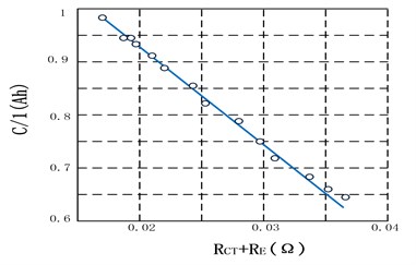
Fig. 3Degradation curve of Li-ion battery capacity

It can be seen from the above experimental data, at the beginning of the prediction, the number of historical data is limited, so it is still strict with the predictive modeling method and demanding because of interference or man-made wrong operation in the experiment, as well as some abnormal data in the data set. Thus, it is necessary to carry out the raw data preprocessing on the abnormal data points firstly. Since the number of charge and discharge cycles of lithium-ion batteries has reached 500 to 700, and many corresponding test data points can reduce the calculation efficiency. Thus, the degradation trend of Li-ion battery can obtain 8 data. For example, simplify the original data and return one data reduction data every 5 data intervals. The degradation trend of is consistent with the original data obviously. In order to evaluate the prediction accuracy, the definition is as follows:

where, $RU{L}_{\mathrm{A}\mathrm{c}\mathrm{t}\mathrm{u}\mathrm{a}\mathrm{l}\mathrm{v}\mathrm{a}\mathrm{l}\mathrm{u}\mathrm{e}}$ is the true RUL of the Li-ion battery, and $RU{L}_{\mathrm{P}\mathrm{r}\mathrm{e}\mathrm{d}\mathrm{i}\mathrm{c}\mathrm{t}\mathrm{i}\mathrm{v}\mathrm{e}\mathrm{v}\mathrm{a}\mathrm{l}\mathrm{u}\mathrm{e}}$ is the RUL value predicted by the model method.

3. GA optimize LM-BPNN modeling

4. Prediction of li-ion battery based on GA-LM-BPNN

4.2. Research on BPNN prediction

Carry out 100 debugging for the parameters of three-layer BP network, and determine that the number of iterations is set as 100, the learning rate is set as 0.1, and the training target is set as 0.004 %. The test data are filtered, and the noise signal is removed and normalized. 2000 groups of data are randomly selected, 1900 groups are used as training data, and 100 groups are used as test data. Then, the test set is input into the BPNN model to predict the output, and the result is shown in Fig. 4. For the selected test data set, the error is shown in Fig. 4.

It is not difficult to see from Fig. 4 that the overall output result of BPNN is quite good, but there is still some prediction error, mainly concentrated in the initial stage of prediction. The error is still a little large, and the maximum reaches 0.0297.

Fig. 4Predict error of BPNN

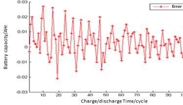
Fig. 5Predict error of BPNN samples

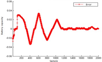
It is not difficult to see from Fig. 5 that the overall prediction effect is good when training samples are learned according to the structure of BPNN. The maximum error is 0.03. After the training samples reach 1200, the prediction error becomes smaller and smaller, which is relatively stable with little fluctuation.

4.3. Prediction of LM-BPNN by GA optimization

Firstly, the structure of BPNN is 5-6-1. Then code length of the GA individual is 42 bits; the evolutionary algebra of GA is 50, and the population size is set as 30. The crossover operation sets conducted by the roulette method. The crossover probability is set as 0.8; the mutation probability is 0.01, and the fitness error function is $F$. According to the steps of GA-LM-BPNN, the curve of fitness function changes in the GA optimization process decreases with the increase of algebra. It indicates that the prediction error is getting smaller and smaller, and the optimal weights and thresholds obtained after 50 generations, which are shown in Table 2.

Table 2Optimal weights and threshold

${\mathrm{\omega }}_{\mathrm{m}\mathrm{i}}$	1.4819	1.4931	–2.7276	–2.2447	–0.9881	–1.9257
	–0.9496	–2.5244	1.8420	–2.5901	–0.0168	–2.0345
	1.0456	–0.5914	–2.0804	–0.0187	0.9711	1.5852
	–1.3385	-0.3675	1.0724	1.1690	0.9329	–1.7788
	–2.7230	-0.7106	1.5464	1.5931	–1.9729	1.8532
${\mathrm{a}}_{\mathrm{i}}$	1.7532	1.7712	1.4588	–0.3265	–0.0877	0.2911
${\mathrm{\omega }}_{\mathrm{i}\mathrm{p}}$	2.8814	–1.1865	0.6284	–2.1562	–0.4892	1.3088
${\mathrm{b}}_{\mathrm{p}}$	–0.6668	–	–	–	–	–

Fig. 6Predict result of GA-LM-BP network

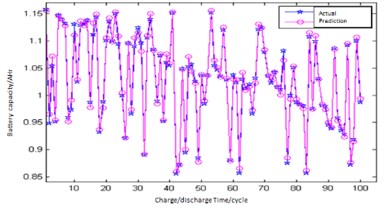
Fig. 7Predict error of GA-LM-BP network

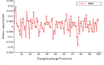
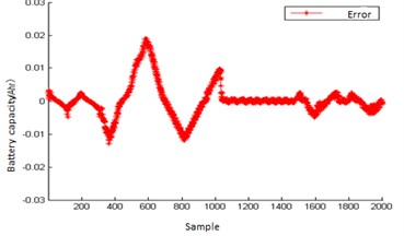
The optimal weights and thresholds are assigned to BPNN, and the optimized network is used to train. Then the output of the whole system is predicted, as shown in Fig. 6, Fig. 7.

It is not difficult to see from Fig. 6 and Fig. 7 that GA-LM-BPNN is more capable than BPNN in fitting nonlinear functions, with significantly reduced prediction errors and improved accuracy. From Fig. 8 and Fig. 9, GA-LM-BPNN has better output prediction effect, with the highest prediction error of 0.0195 and the average error of 0.0045. By comparing the prediction output effect of BPNN and GA-LM-BPNN, the prediction result is more accurate and the stability is improved after the initial weight and threshold value are optimized by GA. The prediction error is significantly improved and the global convergence is good.

Fig. 8Predict output of GA-LM-BP network

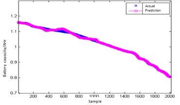
Fig. 9Predict error of GA-LM-BP network

5. Conclusions

The LM algorithm and GA algorithm are introduced into BP neural network algorithm. It not only combines the rapidity of gauss-Newton method and gradient descent method, but also optimizes the initial weight and threshold of BP neural network to reduce the probability of falling into the local minimum. Fuel by increasing computer power and algorithmic advances, machine learning techniques have become powerful tools for finding patterns of data. The field of quantum machine learning explores how to devise and implement quantum software that could enable machine learning faster than that of classical computers. The application in the prediction of Lithium-ion batteries will have a huge effect.

References

-
Z. S. Zhang, “Research on modeling and fault prediction of Li-ion batteries,” Master’s Thesis, Dalian Maritime University, 2016.
H. C. Dong, “Research on diagnosis method of satellite power battery health,” Ph.D. Thesis, Harbin Institute of Technology, 2015.
Y. Miao, P. Hynan, A. Von Jouanne, and A. Yokochi, “Current Li-ion battery technologies in electric vehicles and opportunities for advancements,” Energies, Vol. 12, No. 6, p. 1074, Mar. 2019, https://doi.org/10.3390/en12061074
W. Li, K. R. Crompton, C. Hacker, and J. K. Ostanek, “Comparison of current interrupt device and vent design for 18650 format lithium-ion battery caps,” Journal of Energy Storage, Vol. 32, p. 101890, Dec. 2020, https://doi.org/10.1016/j.est.2020.101890
G. Yang and W. Yu, “Eddy current damper capable of collecting electric energy,” Vibroengineering PROCEDIA, Vol. 33, pp. 28–33, Oct. 2020, https://doi.org/10.21595/vp.2020.21672
B. Saha, K. Goebel, and J. Christophersen, “Comparison of prognostic algorithms for estimating remaining useful life of batteries,” Transactions of the Institute of Measurement and Control, Vol. 31, No. 3-4, pp. 293–308, Jun. 2009, https://doi.org/10.1177/0142331208092030
About this article
This work is supported by the National Defense Preresearch Foundation 9140A27020113JB11393 and 9140A27020314JB11438.