Gearbox fault diagnosis through quantum particle swarm optimization algorithm and kernel extreme learning machine

Meng, Shuo; Kang, Jianshe; Chi, Kuo; Die, Xupeng

doi:10.21595/jve.2020.21550

Journal of Vibroengineering

Browse Journal

Submit article

Published: 15 September 2020

Check for updates

Gearbox fault diagnosis through quantum particle swarm optimization algorithm and kernel extreme learning machine

Shuo Meng¹

Jianshe Kang²

Kuo Chi³

Xupeng Die⁴

^{1, 2, 3, 4}Shijiazhuang Branch, Army Engineering University, Shijiazhuang, China

Corresponding Author:

Shuo Meng

Cite the article Download PDF

Downloads 1086

WoS Core Citations 5

CrossRef Citations 6

Abstract

Gearbox is the key component of mechanical transmission system. Accurate fault diagnosis of gearbox is of great significance to ensure the operation of rotating machinery. Based on the comprehensive simulation test-bed in the laboratory, a gearbox fault diagnosis method based on QPSO-KELM is proposed. Firstly, the fault pre planting experiments of gear fault, bearing fault and gear bearing mixed fault are carried out on the comprehensive simulation test-bed. Then, the vibration signals collected are preprocessed by TSA to eliminate noise. The time domain, frequency domain and NASA feature parameters of the preprocessed signals are taken as training samples and test samples of QPSO-KELM. The experimental results show that the proposed method can effectively solve the problem of gearbox fault pattern recognition, and the fault diagnosis accuracy is higher than traditional methods, so the research has certain reference significance and engineering application value.

Gearbox fault diagnosis through quantum particle swarm optimization algorithm and kernel extreme learning machine

1. Introduction

Gearbox is widely used in fans, machine tools, vehicles and other equipments. As a key component of mechanical transmission system, gearbox will cause huge economic losses and even casualties in case of failure during equipment operation. Therefore, the earlier the fault is found in the gearbox and the earlier the maintenance is carried out, the more loss can be reduced. The main components of gearbox are shaft, bearing and gear, among which gear failure and bearing failure are quite common.

At present, the mechanical transmission system fault diagnosis research is extensive, and the method is diverse. As the most mainstream classification method, intelligent classification algorithm has achieved good results in the field of equipment fault diagnosis. Common intelligent classification algorithms include neural network [1, 2], support vector machine (SVM) [3-5], kernel extreme learning machine (KELM) [6, 7], deep learning [8-10] and other methods. Wang [2] proposed a fault diagnosis method based on RDGWPR-MSE and PNN, which is used to realize the automatic fault identification of electric submersible pump. Wang and Yan [4] used the energy of IMF component after SVD decomposition as feature parameters to input and train SVM model, so as to realize bearing fault diagnosis. Saari et al. [5] proposed a fault diagnosis method for wind turbine bearing based on one class SVM. Iosifidis A et al. [7] studied the classification method of KELM, and achieved good results. Yang Yu et al. [9] proposed a structure adaptive DBN algorithm to solve the problem of difficult to determine the structure of DBN, which was successfully applied to the fault classification of rolling bearings. Shao et al. [10] successfully diagnosed the bearing fault by combining the dual tree complex wavelet packet transform with the adaptive DBN algorithm.

Compared with these methods, KELM has a stronger comprehensive advantage in sample size, network generalization, calculation speed and accuracy, so KELM is more suitable for solving gearbox fault diagnosis problems that require higher calculation speed and accuracy. Since the classification capability of KELM network is greatly affected by the value of kernel parameters and penalty coefficient, it is necessary to optimize the above structure parameters. Currently, genetic algorithm [11], fish swarm algorithm [12], whale algorithm[13], ant colony algorithm [14], wolf algorithm [15], particle swarm algorithm [16] and other intelligent algorithms have been widely applied in the field of parameter optimization, such as Xu [13] used whale algorithm to optimize wavelet kernel extreme learning machine (WKELM) and Wang [17] used the modified WKELM wolves algorithm in diagnosing rolling bearing fault; Wu [18] used ant colony algorithm for fault diagnosis of rotating mechanical equipment. Pei [19] used particle swarm optimization algorithm to optimize KELM for transformer fault diagnosis. Liu [20] proposed the method of combining the variational mode decomposition (VMD) with the improved KELM for engine fault diagnosis. However, most of the above parameter optimization methods have the problem of long calculation time and easy to fall into the local optimum. Therefore, the QPSO-KELM (KELM-based on Quantum Particle Swarm Optimization) [21-23] was put forward. With strong global search ability, the QPSO can find the optimal parameters of KELM, thereby, the learning speed and classification accuracy of KELM can be improved and the accuracy of gearbox fault diagnosis will also be improved.

2. Fault diagnosis strategy of gearbox based on QPSO-KELM

The fault diagnosis process of gearbox based on QPSO-KELM is described as follows:

(1) Signal acquisition. In general, the closer the sensor is to the source of the vibration, the better the signal will be.

(2) Extract the fault characteristic parameters. The time-domain characteristic parameters, frequency-domain characteristic parameters and the characteristic parameters in the technical report of NASA were extracted from the collected signals. Then, the corresponding training set and test set were selected from all samples in a ratio of 3:1.

(3) The training of KELM. Aiming at maximizing the training accuracy, the training set is input to KELM, and the QPSO algorithm is used to search the optimal parameters. After that, the trained KELM can be obtained.

(4) Calculate the test accuracy. Input the test samples to the trained KELM, the correct classification times of test samples will be calculated and the test accuracy will be calculated.

The above process is shown in Fig. 1.

Fig. 1The process of fault diagnosis of gearbox based on QPSO-KELM

In the Fig. 1, the gearbox fault diagnosis process also involves time-domain synchronous average algorithm [24], time-domain synchronous resampling algorithm [25, 26], pre-whitening algorithm [27], relevant fault characteristic parameters, KELM, QPSO and other relevant contents.

2.1. Signal preprocessing

During the signal acquisition process, the signal are easy interfered by other vibration signals, such as the vibration of the bearing of the equipment itself, the vibration of the motor, the meshing vibration of the gear independent of the synchronous shaft and the vibration from other machines and equipment. As a signal preprocessing technology, time synchronous averaging (TSA) technology can eliminate the signal components irrelevant to the synchronous shaft and enhance the fault signals of the synchronous shaft gear and its meshing gear, making the gear fault diagnosis easier. Where, the reference axis is the synchronous axis and the non-reference axis is the nonsynchronous axis. The theoretical equation of TSA is as follows:

1

y_{n} = \frac{1}{M} \sum_{m = 0}^{M - 1} x_{n + m N}, n = 1, \dots N,

where, $y_{n}$ is the TSA signal, $x$ is the original signal, and $M$ is the average times.

In the actual process, the implementation steps of TSA are as follows:

(1) Determine the zero crossing point of the synchronous axis according to the speed pulse signal, that is, the starting or ending position of each rotation of the synchronous axis.

(2) According to the position of zero crossing, divide the vibration acceleration signal into $M - 1$ segments, and each segment represents the sampling signal of the integer rotation of the synchronous axis.

(3) Perform cubic curve interpolation for each signal segment, so that the sampling points of each signal segment are the same. The newly interpolated sampling points are $n = 2^{c e i l i n g (l o g 2 (g))}$ , where $g$ is the mean of sampling points of each signal segment.

(4) Stack and average the resampled signals to obtain the time-domain synchronous average signal.

Based on the speed signal sampled at the same angle, TSA resamples the time-domain vibration acceleration signal to ensure that each revolution has the same number of sampling points, that is, equal angle sampling. The speed signal is usually obtained by the photoelectric sensor, and a rotation of the axis produces several pulses. The more pulses generated by a rotation, the more accurate the speed signal will be. The position of zero crossing can be obtained by rotating speed signal, and it is the key of the TSA algorithm. The gear fault data is mainly the fault characteristic parameters extracted from the time-domain synchronous average signal.

2.2. Extract feature parameters [28]

After preprocessing, the feature extraction of the preprocessed signal is carried out. The feature parameters are the basis for feature classification and fault recognition. The feature parameters adopted in this paper include time-domain feature parameters, frequency-domain feature parameters and some feature parameters mentioned in the report of NASA.

Time-domain characteristic parameters include: maximum ( $X_{1}$ ), minimum ( $X_{2}$ ), peak-to-peak ( $X_{3}$ ), mean value ( $X_{4}$ ), mean square value ( $X_{5}$ ), root mean square ( $X_{6}$ ), variance ( $X_{7}$ ), standard deviation ( $X_{8}$ ), energy ( $X_{9}$ ), root square amplitude ( $X_{10}$ ), mean square amplitude ( $X_{11}$ ), mean square amplitude ( $X_{12}$ ), kurtosis ( $X_{13}$ ), skewness ( $X_{14}$ ), waveform index ( $X_{15}$ ), peak index ( $X_{16}$ ), pulse index (X₁₇), margin index ( $X_{18}$ ), clearance coefficient ( $X_{19}$ ), etc:

X_{1} = m a x (x_{i}), X_{2} = m i n (x_{i}), X_{3} = x_{m a x} - x_{m i n}, X_{4} = \frac{1}{N} \sum_{i = 1}^{N} x_{i},

X_{5} = \frac{1}{N} \sum_{i = 1}^{N} x_{i}^{2}, X_{6} = \sqrt{\frac{1}{N} \sum_{i = 1}^{N} x_{i}^{2}}, X_{7} = m a x |x_{i}|, X_{8} = \frac{1}{N} \sum_{i = 1}^{N} {(x_{i} - X_{4})}^{2},

X_{9} = \sqrt{\frac{1}{N} \sum_{i = 1}^{N} {(x_{i} - X_{4})}^{2}}, X_{10} = \sum_{i = 1}^{N} x_{i}^{2}, X_{11} = \frac{\frac{1}{N} \sum_{i = 1}^{N} {(x_{i} - X_{4})}^{3}}{X_{6}^{3}},

X_{12} = \frac{\frac{1}{N} \sum_{i = 1}^{N} {(x_{i} - X_{4})}^{4}}{X_{6}^{4}}, X_{13} = {(\frac{1}{N} \sum_{i = 1}^{N} {|x_{i}|}^{1 / 2})}^{2}, X_{14} = \frac{1}{N} \sum_{i = 1}^{N} |x_{i}|,

X_{15} = \frac{X_{6}}{|X_{14}|}, X_{16} = \frac{X_{7}}{X_{6}}, X_{17} = \frac{X_{7}}{X_{14}}, X_{18} = \frac{X_{7}}{X_{13}}, X_{19} = \frac{X_{1}}{X_{3}} .

Some common statistical features in the frequency domain are shown below. Feature $p_{1}$ namely mean frequency. Features $p_{2}$ - $p_{4}$ , $p_{6}$ , and $p_{11}$ - $p_{13}$ describe the convergence of the spectrum power, reflecting the energy of frequency spectrum. Features $p_{5}$ and $p_{7}$ - $p_{9}$ show the change of main frequencies which are dominant in the frequency spectrum. The features in frequency-domain are calculated from the spectrum of the original signal, which contains more effective information than time-domain features:

p_{1} = X_{m f} = \frac{\sum_{k = 1}^{K} s (k)}{K}, p_{2} = \frac{\sum_{k = 1}^{K} (s (k) - p_{1})^{2}}{K - 1}, p_{3} = \frac{\sum_{k = 1}^{K} (s (k) - p_{1})^{3}}{K (\sqrt{p_{2}})^{3}},

p_{4} = \frac{\sum_{k = 1}^{K} ((s (k) - p_{1}))^{4}}{K {p_{2}}^{2}}, p_{5} = X_{f c} = \frac{\sum_{k = 1}^{K} f_{k} s (k)}{\sum_{k = 1}^{K} s (k)}, p_{6} = \sqrt{\frac{\sum_{k = 1}^{K} (f_{k} - p_{5})^{2} s (k)}{K}},

p_{7} = X_{r m s f} = \sqrt{\frac{\sum_{k = 1}^{K} {f_{k}}^{2} s (k)}{\sum_{k = 1}^{K} s (k)}}, p_{8} = \sqrt{\frac{\sum_{k = 1}^{K} {f_{k}}^{4} s (k)}{\sum_{k = 1}^{K} {f_{k}}^{2} s (k)}}, p_{9} = \frac{\sum_{k = 1}^{K} {f_{k}}^{2} s (k)}{\sqrt{\sum_{k = 1}^{K} s (k) \sum_{k = 1}^{K} {f_{k}}^{4} s (k)}},

p_{10} = \frac{p_{6}}{p_{5}}, p_{11} = \frac{\sum_{k = 1}^{K} (f_{k} - p_{5})^{3} s (k)}{K {p_{6}}^{3}}, p_{12} = \frac{\sum_{k = 1}^{K} (f_{k} - p_{5})^{4} s (k)}{K {p_{6}}^{4}},

p_{13} = \frac{\sum_{k = 1}^{K} (f_{k} - p_{5})^{1 / 2} s (k)}{K \sqrt{p_{6}}}, p_{14} = \sqrt{\frac{\sum_{k = 1}^{K} (f_{k} - p_{5})^{2} s (k)}{\sum_{k = 1}^{K} s (k)}} .

In addition to the common time-domain and frequency-domain features, NASA also proposed some features, such as FM0, ER, FM4, FM4*, M6A, M6A*, M8A, M8A*, NA4, NA4*, NB4, NB4*, ER, EOP, etc. These features are mainly used to assess the gear failure:

F M 0 = \frac{P P_{x}}{\sum_{n = 0}^{H} P_{n}}, F M 4 = \frac{N \sum_{i = 1}^{N} {(d_{i} - \bar{d})}^{4}}{{[\sum_{i = 1}^{N} {(d_{i} - \bar{d})}^{2}]}^{2}}, F M 4^{*} = \frac{1 / N \sum_{i = 1}^{N} {(d_{i} - \bar{d})}^{4}}{{[1 / M^{'} \sum_{j = 1}^{M^{'}} 1 / N \sum_{k = 1}^{N} {(d_{j k} - {\bar{d}}_{j})}^{2}]}^{2}},

M 6 A = \frac{N^{2} \sum_{i = 1}^{N} {(d_{i} - \bar{d})}^{6}}{{[\sum_{i = 1}^{N} {(d_{i} - \bar{d})}^{2}]}^{3}}, M 6 A^{*} = \frac{1 / N \sum_{i = 1}^{N} {(d_{i} - \bar{d})}^{6}}{{[1 / M^{'} \sum_{j = 1}^{M^{'}} 1 / N \sum_{k = 1}^{N} {(d'_{j k} - \bar{d}'_{j})}^{2}]}^{3}},

M 8 A = \frac{N^{3} \sum_{i = 1}^{N} {(d_{i} - \bar{d})}^{8}}{{[\sum_{i = 1}^{N} {(d_{i} - \bar{d})}^{2}]}^{4}}, M 8 A^{*} = \frac{1 / N \sum_{i = 1}^{N} {(d_{i} - \bar{d})}^{8}}{{[1 / M^{'} \sum_{j = 1}^{M^{'}} 1 / N \sum_{k = 1}^{N} {(d'_{j k} - \bar{d}'_{j})}^{2}]}^{4}},

N A 4 = \frac{N \sum_{i = 1}^{N} {(r_{i} - \bar{r})}^{4}}{{[1 / M \sum_{j = 1}^{M} \sum_{k = 1}^{N} {(r'_{j k} - \bar{r}'_{j})}^{2}]}^{2}}, N A 4^{*} = \frac{1 / N \sum_{i = 1}^{N} {(r_{i} - \bar{r})}^{4}}{{[1 / M_{1} \sum_{j = 1}^{M_{1}} \sum_{k = 1}^{N} {(r'_{j k} - \bar{r}'_{j})}^{2}]}^{2}},

N B 4 = \frac{1 / N \sum_{i = 1}^{N} {(s_{i} - \bar{s})}^{4}}{{[1 / M \sum_{j = 1}^{M} 1 / N \sum_{k = 1}^{N} {(s_{j k} - {\bar{s}}_{j})}^{2}]}^{4}} \bar{s}, N B 4^{*} = \frac{1 / N \sum_{i = 1}^{N} {(s_{i} - \bar{s})}^{4}}{{[1 / M' \sum_{j = 1}^{M'} 1 / N \sum_{k = 1}^{N} {(s_{j k} - {\bar{s}}_{j})}^{2}]}^{4}},

E R = \frac{R M S_{d_{i}}}{R M S_{d_{i}^{'}}} = \sqrt{\frac{1 / N \sum_{i - 1}^{N} (d_{i})^{2}}{1 / N \sum_{i - 1}^{N} ({d_{i}}^{'})^{2}}}, E O P = \frac{N \sum_{i = 1}^{N} {(r e_{i} - \bar{r} \bar{e})}^{4}}{{[\sum_{i = 1}^{N} {(r e_{i} - \bar{r} \bar{e})}^{2}]}^{2}} .

3. Research on classification method based on QPSO-KELM

3.1. KELM

In KELM algorithm, the kernel function is introduced into ELM, and the input weights and offsets in ELM are replaced by kernel function mapping, which makes the output of the ELM more stable and solves the over learning problems. Therefore, the KELM is widely used in classification identify areas.

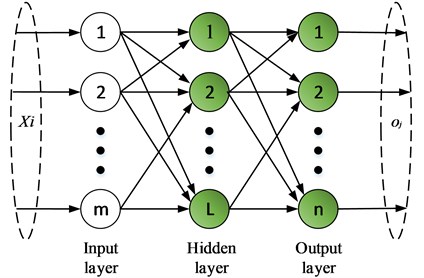
ELM is a single hidden layer feedforward neural network, and its hidden layer weight does not need to be adjusted by feedback regulation. The structure of the ELM is shown in the Fig. 2, including an input layer, a hidden layer and an output layer.

Suppose $Z = {x_{i}, t_{i}}_{i = 1}^{N}$ are $N$ training sample sets, where $x_{i} = [x_{i 1}, x_{i 1}, \dots, x_{i m}]^{T} \in R^{m}$ is the input characteristic parameter and $t_{i} = [t_{i 1}, t_{i 1}, \dots, t_{i n}]^{T} \in R^{n}$ is the sample label, then the output function expression of ELM training model is:

2

\sum_{i = 1}^{M} β_{i} g (w_{i} \cdot x_{i} + b_{i}) = o_{i}, i = 1,2, \dots, N,

where, $w_{i} = [w_{1 i}, w_{2 i}, \dots, w_{m i}]$ and $β_{i} = [β_{i 1}, β_{i 2}, \dots, β_{i n}]^{T}$ represent the input and output weight matrix of the $i$ th hidden layer node respectively; $o_{j} = [o_{i 1}, o_{i 2}, \dots, o_{i n}]^{T}$ represents the output layer vector of the ELM.

Fig. 2ELM model

The goal of ELM training is to make the error between the actual output of the training sample and the sample label close to 0, the equation is:

3

\sum_{i = 1}^{N} ‖o_{i} - t_{i}‖ = 0, β_{i} w_{i} b_{i} \sum_{i = 1}^{M} β_{i} g (w_{i} \cdot x_{i} + b_{i}) = t_{i}, i = 1,2, \dots, N, H β = T .

So the existence of $β_{i}$ , $w_{i}$ and $b_{i}$ can be used to obtain the Eq. (4), as below:

4

\sum_{i = 1}^{M} β_{i} g (w_{i} \cdot x_{i} + b_{i}) = t_{i}, i = 1,2, \dots, N .

The Eq. (4) can be expressed as a matrix:

5

H β = T,

where, $H$ is the output matrix of the hidden layer, which can be expressed in the following equation:

6

H (w_{1}, \dots, w_{M}, b_{1}, \dots, b_{M}, x_{1}, \dots, x_{N}) = {[\begin{matrix} g (w_{1} \cdot x_{1} + b_{1}) & \dots & g (w_{M} \cdot x_{1} + b_{M}) \\ ⋮ & \dots & ⋮ \\ g (w_{1} \cdot x_{N} + b_{1}) & \dots & g (w_{M} \cdot x_{N} + b_{M}) \end{matrix}]}_{N \times M},

7

β = {[\begin{array}{l} β_{1}^{T} \\ ⋮ \\ β_{M}^{T} \end{array}]}_{M \times n}, T = {[\begin{array}{l} t_{1}^{T} \\ ⋮ \\ t_{N}^{T} \end{array}]}_{N \times n} .

For $β$ , the equation is as follows:

8

β^{'} = H^{+} T,

where, $H^{+}$ represents the inverse matrix of $H$ , $β^{'}$ is the optimal quadratic solution to $β$ .

According to the structural optimization and ERM criteria, the output weight $β$ of ELM can be determined, that is:

9

\begin{array}{l} M i n i m i z e : L_{P_{E L M}} = \frac{1}{2} {‖β‖}^{2} + C \frac{1}{2} \sum_{i = 1}^{N} {‖ξ_{i}‖}^{2}, \\ S u b j e c t t o : h (x_{i}), β = t_{i}^{T} - ξ_{i}^{T}, i = 1, \dots, N, \end{array}

where, $ξ_{i} = {[ξ_{i, 1}, \dots, ξ_{i, m}]}^{T}$ represents network calculation error, $\frac{1}{2} {‖β‖}^{2}$ is the structural error, $\frac{1}{2} {\sum_{p = 1}^{N} ‖ξ_{p}‖}^{2}$ is the empirical error, and $C$ is the penalty factor.

Through the optimization of the solution, the optimal solution of $β$ can be obtained as follows:

10

β = H^{T} {(\frac{I}{C} + H H^{T})}^{- 1} T .

Therefore, the output model function of ELM is as follows:

11

o_{i} = h_{i} H^{T} {(\frac{I}{C} + H H^{T})}^{- 1} T .

By using kernel operation to replace matrix operation $H$ in ELM, the KELM classification model can be established. The kernel matrix is defined as:

12

Ω = H H^{T} : Ω_{i, j} = h (x_{i}) \cdot h (x_{j}) = K (x_{i}, x_{j}),

where $Ω$ is the symmetric matrix of $N \times N$ and $K (x, y)$ is the kernel function.

Eq. (11) can be expressed by kernel function as follows:

13

o_{i} = [K (x_{i}, x_{j}), \dots, K (x_{i}, x_{j})] λ,

where, $λ$ represents the output weight matrix of KELM.

Different support vector machines can be constructed by selecting different kernel functions. Among the commonly used kernel functions, compared with the polynomial kernel function and Sigmoid kernel function, the radial basis kernel function has the advantages of simple parameters and strong adaptability to randomly distributed samples. Therefore, a SVM based on radial basis kernel function is established in this paper, and its expression is shown as follows:

14

K (x, x_{i}) = e x p (- \frac{{‖x - x_{i}‖}^{2}}{σ^{2}}) .

According to Eq. (9) and (14), it can be seen that KELM contains kernel parameter $σ$ and penalty coefficient $C$ , and it is necessary to find the optimal parameter to make the classification effect of KELM the best.

3.2. QPSO-KELM

By quantizing the iterative updating process of particles of PSO algorithm, the QPSO can reduce the algorithm complexity, improve algorithm convergence speed and global search ability. The basic principles of QPSO are as follows:

Assume that $Ω$ is the $d$ -dimensional search space, and the population number of particles in the space is $b$ , then the position of the $i$ th particle can be expressed as:

15

V_{i} = (v_{i 1}, v_{i 2} \dots v_{i d}) .

Suppose the individual optimal position of the particle is $p_{i b e s t}$ , and the global optimal position of the particle is $p_{g b e s t}$ , the $p_{i b e s t}$ and $p_{g b e s t}$ are as follows:

16

p_{i b e s t} = (p_{i 1}, p_{i 2} \dots p_{i d}),

17

p_{g b e s t} = (p_{g 1}, p_{g 2} \dots, p_{g d}) .

The particle can find and update its individual optimal position $p_{i}$ and population optimal position $p_{g}$ through iterative operation, and the average optimal position $m b e s t$ can be introduced as the population optimal center. Then the particle optimization process can be expressed as:

18

m b e s t = \frac{1}{M} \sum_{i = 1}^{M} p_{i b e s t} = [\frac{1}{M} \sum_{i = 1}^{M} p_{i 1}, \frac{1}{M} \sum_{i = 1}^{M} p_{i 2} \dots \frac{1}{M} \sum_{i = 1}^{M} p_{i d}],

19

p_{i d} = φ p_{i d} + (1 - φ) p_{g d}, φ \in (0,1),

20

v_{i d} = p_{i d} \pm α |m b e s t - v_{i d}| l n (1 / u), u \in (0,1),

where, $α$ is the contraction expansion factor, which is dynamically adjusted in the iterative operation according to the Eq. (21):

21

α = (α_{1} - α_{2}) \times \frac{N - t}{N} + α_{2},

where, $N$ represents the maximum number of iterations. $α_{1}$ and $α_{2}$ are the initial and final values of $α$ respectively, usually the two parameters are set as: $α_{1} = 0.5$ , $α_{2} = 1$ .

According to the basic principle of KELM and QPSO, the network training process which is used QPSO to optimize the network structure parameters of KELM is as follows:

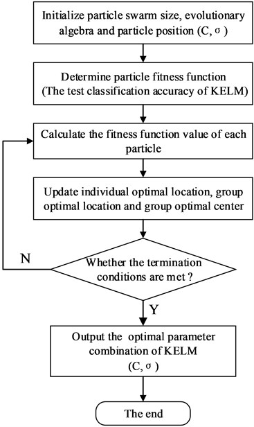
(1) Initialize the position of population particles, and set parameters such as particle swarm size, iteration step size, termination conditions and so on.

(2) Initialize the current position of each particle as $p_{i b e s t}$ , define the classification accuracy of KELM as fitness function, and calculate the fitness value of each particle. The position of the particle with the maximum fitness value was initialized as $p_{g b e s t}$ .

(3) Update the particle position according to Eq. (18-20).

(4) The fitness value of each particle is calculated, and the individual optimal position $p_{b e s t}$ , the group optimal position $p_{g b e s t}$ and the group optimal center $m b e s t$ are updated based on the optimal fitness value.

(5) Judge whether the termination conditions are met. If so, stop the calculation and output the result, if not, return to step (3).

According to the above steps, the modeling flow chart of QPSO-KELM can be drawn as shown in Fig. 3.

Fig. 3Modeling flow chart of QPSO-KELM

4. Experimental verification and discussion

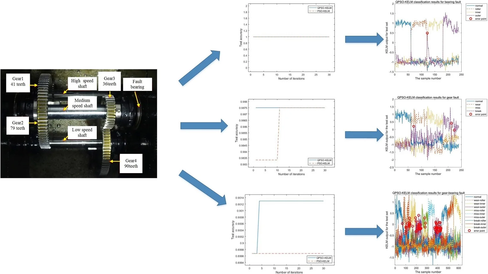
To verify whether the QPSO-KELM is available, the pre planting fault tests are carried out for gear fault, bearing fault and gear-bearing mixed fault. The fault simulation test rig is shown in Fig. 4. The test rig consists of four parts: the power and control part, the bearing fault simulation part (not used), the gear fault simulation part and the data acquisition part (not shown). This section mainly uses the gearbox fault simulation part, which is mainly composed of a two-stage reduction spur gearbox, a magnetic powder brake (supply the load) and a magnetic powder brake controller (control the load change).

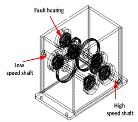
The perspective and internal structure of the two-stage reduction spur gearbox are shown in Fig. 5. The teeth number in the gearbox from high speed shaft to low speed shaft is 41, 79, 36 and 90. The fault gear is the intermediate shaft pinion gear (gear 3 with 36 teeth). The fault types include wear, break and miss teeth. The fault bearing is located in the deep groove ball bearing at the end cover of the gear 3 side of the medium-speed shaft (Fig. 5(b)). The deep groove ball bearing type is ER-16k, and its size parameters are shown in Table 1. The fault types include inner race fault, outer race fault and single roller fault.

Fig. 4The mechanical fault simulation test bench

In the test, we set two vibration acceleration sensors in vertical and horizontal directions respectively. Both sensors are installed outside the end cover of the fault bearing (Fig. 5(c)), which are used to collect the vibration acceleration data in vertical and horizontal directions. The data acquisition parameters are set as: sampling frequency $f s =$ 20.48 kHz, sampling time $t =$ 48 s, motor speed 30 r/s (the actual motor speed is about 29.602 r/s). According to the speed of the motor, the number of gear teeth of the gearbox and the main dimension parameters of the bearing ER-16K (Table 1), the main relevant frequency of the gearbox can be calculated by the calculation formula of bearing fault characteristic frequency (Table 2). The calculation results are shown in Table 3.

Fig. 5The structure of gearbox

a) Perspective view

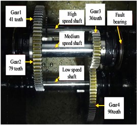
b) The inner structure

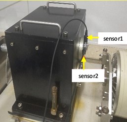
c) The outer structure

4.1. Bearing fault diagnosis

Firstly, the single fault of bearing is analyzed. In the experiment, the motor speed is set to 30 r/s, and the signal sampling frequency is 20.48 kHz. The analysis data is mainly collected by sensor1 (vertical direction). The test data types include bearing normal data, rolling element fault data, inner ring fault data and outer ring fault data, each type contains 240 groups of data, and 960 groups of data is in total. The sampling time of each group of data is 2 seconds.

Table 1Main dimensions of bearing ER-16K

Number of rolling elements $N_{b}$	Ball diameter $d$ / inch	Pitch diameter $D$ / inch	Contact angle $θ$ (°)
9	0.3125	1.516	0

Table 2The formulas of fault characteristic frequencies to bearings

Name	Formulas
Fault characteristic frequencies of outer race	$f_{B P F O} = \frac{N_{b}}{2} f_{r} [1 - \frac{d c o s (θ)}{D}]$
Fault characteristic frequencies of inner race	$f_{B P F I} = \frac{N_{b}}{2} f_{r} [1 + \frac{d c o s (θ)}{D}]$
Fault characteristic frequencies of ball spin	$f_{B S F} = \frac{D}{d} f_{r} [1 - \frac{d^{2} c o s^{2} (θ)}{D^{2}}]$
$N_{b}$ is the number of rolling elements, $d$ means the Ball diameter, $D$ means the Pitch diameter, $θ$ means the Contact angle, $f_{r}$ is the bearing rotation frequency

Table 3Relevant frequencies of the gearbox

Rotating frequency / r∙s^-1			Meshing frequency / Hz		Fault feature frequency of bearing/ Hz
$f_{r 1}$	$f_{r 2}$	$f_{r 3}$	$f_{m 1}$	$f_{m 2}$	$f_{B P F O}$	$f_{B P F I}$	$f_{B S F}$
29.602	15.363	6.145	1213.662	553.061	54.882	82.448	35.681
$f_{r 1}$ is the rotating frequencies of high speed axis, $f_{r 2}$ is the rotating frequencies of medium speed axis, $f_{r 3}$ is the rotating frequencies of low speed axis; $f_{m 1}$ is the meshing frequencies of gear 1 and gear 2, $f_{m 2}$ is the meshing frequencies of gear 3 and gear 4; $f_{B P F O}$ is the fault characteristic frequencies of the bearing outer race, $f_{B P F I}$ is the fault characteristic frequencies of the bearing inner race, $f_{B S F}$ is the fault characteristic frequencies of the bearing ball spin

When diagnosing the bearing fault, follow the procedure shown in Fig. 1. Firstly, the time-domain, frequency-domain and NASA characteristic parameters of the bearing fault were extracted from the bearing data of each group, and 960 samples will be obtained. And each group of the samples is marked with the following rules: normal-1, roller-2, inner-3, outer-4. Then, the training set and test set are selected from all samples in a ratio of 3:1, and the training set is input to KELM for training. In order to maximize the test accuracy, QPSO is used to optimize the parameters of KELM. Finally, in order to verify the superiority and effectiveness of the method, the ELM and PSO-KELM are also applied to bearing fault diagnosis, and the experiment results of different methods are used to compare with each other.

Since the standard elm algorithm uses a single layer feedforward neural network structure, it is unnecessary to consider the parameter optimization of ELM. So the parameter optimization process of PSO-KELM and QPSO-KELM are analyzed, the results is shown in Fig. 6. Therefore, it is only necessary to analyze the parameter optimization process of PSO-KELM and QPSO-KELM.

Fig. 6a) Iterative process of the two methods, b) the local amplify of a)

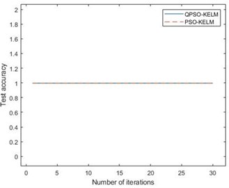
a)

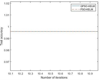
b)

Fig. 6(a) is iterative process of the two methods, Fig. 6(b) is the local amplify of Fig. 6(a). It can be seen from the figure that PSO-KELM and QPSO-KELM algorithm have the highest test accuracy from the beginning, which shows that the fault characteristics of bearing single fault are obvious, and it can achieve high classification accuracy without parameter iteration optimization. The initial parameters setting of QPSO-KELM is $C \in [0.01,1000]$ , $σ \in [0.01,100]$ , and the optomized parameters are $C =$ 1000, $σ =$ 18.

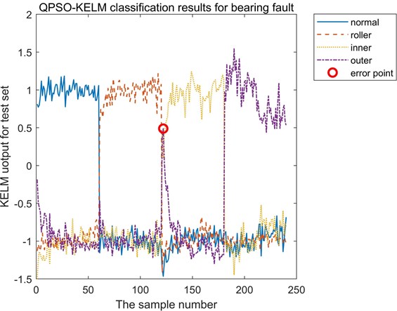
The final training accuracy and test accuracy of the methods are shown in Table 4. It can be seen from Table 4 that both of the training accuracy and the test accuracy of QPSO are the highest and reach 99.58 %. The QPSO-KELM classification results of the test dataset are shown in Fig. 7, in which there is only one misjudgment point, so the accuracy of the trained QPSO-KELM model is reliable.

Table 4Bearing fault classification accuracy

	SVM	CNN	ELM	PSO-KELM	QPSO-KELM
Training accuracy	90.43 %	98.89 %	91.74 %	98.47 %	99.58 %
Testing accuracy	89.97 %	98.74 %	91.74 %	97.92 %	99.58 %

Fig. 7Classification results of bearing test dataset based on QPSO-KELM

4.2. Gear fault diagnosis

Secondly, the single fault of gear is analyzed. The fault gear is the medium-speed shaft pinion in the gearbox, which is gear 3 in Fig. 5(b). In the experiment, the motor speed and the signal sampling frequency are the same as in section 4.1. The analysis data is mainly collected by sensor 1 (vertical direction). The test data types include gear normal data, worn teeth data, broken tooth data and missing tooth data, each type contains 240 groups of data, and 960 groups of data is in total. The sampling time of each group of data is 2 seconds.

When diagnosing the gear fault, follow the procedure shown in Fig. 1. Firstly, the characteristic parameters of gear fault in time-domain, frequency-domain and NASA are extracted from each group of gear data, and 960 samples will be gotten. And each group of the samples is marked with the following rules: normal-1, wear-2, miss-3, break-4. Then, the training set and test set are selected from all samples in a ratio of 3:1, and the training dataset is input to KELM for training. In order to maximize the test accuracy, QPSO is used to optimize the parameters of KELM. Finally, in order to verify the effectiveness of the method and highlight the advantages of the proposed method. The ELM and PSO-KELM are also used for gear fault diagnosis to compare with QPSO-KELM.

The parameters optimization of PSO-KELM and QPSO-KELM are analyzed, the iteration process is shown in Fig. 8. It can be seen from the figure that the QPSO-KELM algorithm has the highest test accuracy from the beginning, which indicates that the QPSO-KELM has stronger learning ability, while PSO-KELM reaches the maximum value at the 11th iteration, which indicates that its learning ability is slightly inferior to the method proposed in this paper. The initial setting of parameters is the same as that in Section 4.1, and the settings after parameter optimization are as follows: $C =$ 1000, $σ =$ 19.

The final training accuracy and test accuracy of the methods are shown in Table 5. It can be seen from Table 5 that both of the training accuracy and the test accuracy of QPSO are the highest and the test accuracy reaches 98.75 %. The QPSO-KELM classification results of the test dataset are shown in Fig. 9, in which there are only three error points, so the accuracy of the trained QPSO-KELM model is available. From the iteration process and fault diagnosis accuracy, it can be seen that the fault features of bearing are more obvious than that of gear. Therefore, gear fault diagnosis needs less iteration times, but higher test accuracy can be achieved.

Fig. 8Iterative process of the two methods

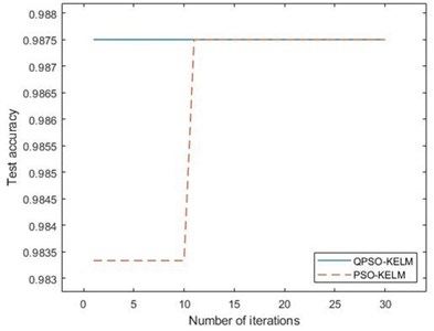
Fig. 9Classification results of gear test dataset based on QPSO-KELM

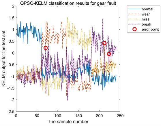
Table 5Gear fault classification accuracy

	SVM	CNN	ELM	PSO-KELM	QPSO-KELM
Training accuracy	83.41 %	98.43 %	80.88 %	98.75 %	99.31 %
Testing accuracy	81.57 %	97.69 %	80.88 %	97.92 %	98.75 %

4.3. Gear-bearing fault diagnosis

At last, the composite faults of gear-bearing are analyzed. The fault parts are the gear and bearing mentioned in the previous section. There are 10 types of gear-bearing data: normal gear-normal bearing data, worn gear – faulty bearing rolling element data, worn gear-faulty bearing inner race data, worn gear-faulty bearing outer race data, gear tooth missing-faulty bearing rolling element data, missing gear tooth-faulty bearing inner race data, missing gear tooth-faulty bearing outer race data, broken gear tooth-faulty bearing rolling element data, broken gear tooth-faulty bearing inner race data, broken gear tooth-faulty bearing inner race data. The mixed faults of gear-bearing is shown in Table 6.

In the experiment, the motor speed is set to 30 r/s, and the signal sampling frequency is 20.48 kHz. The sampling time of each group of data is 2 seconds. The total data is 2472, except the data of the normal state (sample size is 288) and the broken tooth- faulty inner race (sample size is 264), the sample sizes of the other states are all 240 of each group.

Table 6The mixed faults of gear-bearing

Combinations	Gear fault				Bearing fault
Combinations	Normal	Wear	Miss	Break	Normal	Roller	Inner	Outer
1	+				+
2		+				+
3		+					+
4		+						+
5			+			+
6			+				+
7			+					+
8				+		+
9				+			+
10				+				+

When diagnosing the gear-bearing fault, follow the procedure shown in Fig. 1. Firstly, the feature parameters of gear-bearing fault in time-domain, frequency-domain and NASA are extracted from each group of gear-bearing data, and 2742 samples will be gotten. Each group of samples is labeled with the following rules: normal-1, wear-roller-2, wear-inner-3, wear-outer-4, miss-roller-5, miss-inner-6, miss-outer-7, break-roller-8, break-inner-9, break-outer-10. Then, the training set and test set are randomly selected from all samples in a ratio of 3:1, and the training dataset is input to KELM for training. In order to maximize the test accuracy, QPSO is used to optimize the parameters of KELM. Finally, in order to verify the effectiveness of the method and the superiority of the method, the ELM and PSO-KELM are also used for gear-bearing fault diagnosis to compare with QPSO-KELM.

The optimization process of PSO-KELM and QPSO-KELM are shown in Fig. 10. It can be seen from the figure that the test progress of QPSO-KELM algorithm reach the highest after six iterations, while the PSO-KELM algorithm has no transformation from the beginning, and the accuracy is low, indicating that the classification ability of PSO-KELM is weaker than that of QPSO-KELM. The initial setting of parameters is the same as that in Section 4.1, and the settings after parameter optimization are as follows: $C =$ 1000, $σ =$ 20.

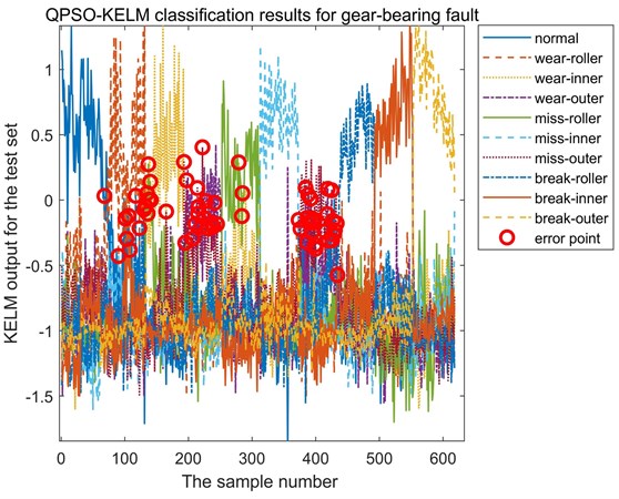
The final classification accuracy of the three methods for mixed faults of gear-bearing is shown in Table 7. It can be seen from Table 7 that the training accuracy of QPSO is not the highest in the training process, but when comparing the final test accuracy, the classification accuracy of QPSO is far higher than that of the other two calculations, and the test accuracy is 90.13 %. However, the test accuracy of the other two methods are no higher than 60 %. The QPSO-KELM classification results of the test dataset are shown in Fig. 11. As can be seen from Fig. 11, the error points are mainly concentrated in three states: the worn-rolling element fault state, worn-outer race fault state and broken-outer race fault state. Therefore, more sensitive feature parameters should be extracted for these three states.

Fig. 10Iterative process of the two methods

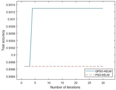
Table 7Classification accuracy of mixed faults of gear-bearing

	SVM	CNN	ELM	PSO-KELM	QPSO-KELM
Training accuracy	58.43 %	90.67 %	53.34 %	92.27 %	92.45 %
Testing accuracy	55.52 %	89.49 %	53.34 %	89.64 %	90.13 %

Fig. 11Classification results of gear-bearing test dataset based on QPSO-KELM

5. Conclusions

A novel QPSO-KELM method is proposed in this paper and applied to gearbox fault diagnosis. The method is implemented by using QPSO algorithm to select the proper KELM parameters, kernel parameter $σ$ and penalty coefficient $C$ . In order to verify the effectiveness and the superiority of the method, the time-domain, frequency-domain and NASA features are collected, the results of the bearing single fault, gear single fault and gear-bearing fault are analyzed. After comparing with two other methods (ELM and PSO-KELM), and analyzing the test results, the following conclusions can be given: (1) Experimental results show that the proposed method is effective, it can identify the types of faults mentioned above; (2) Compared with SVM, ELM, CNN and PSO-KELM, OPSO-KELM has more advantages. The accuracy of QPSO-KELM is more than 90 % in both training data and test data, which is higher than other methods.

The study focuses on optimizing the structural parameters of KELM and the application in gearbox fault diagnosis. From the analysis of experimental results, however, it can be found that there is still a space to improve the identification accuracy of gear-bearing hybrid fault. Since the accuracy of fault judgment is closely related to fault feature extraction, in order to further improve the fault identification accuracy of composite faults, the next step of the study is to extract more sensitive and effective fault feature parameters.

References

Qu Jianling, Yu Lu, Yuan Tao Adaptive fault diagnosis algorithm for rolling bearing based on one-dimensional convolutional neural network. Chinese Journal of Scientific Instrument, Vol. 39, Issue 7, 2018, p. 134-143.

Search CrossRef
Wang Yakun A diagnosis method for electrical submersible pump based on RSGWPT-MSE and PNN. Mechanical Engineer, Vol. 1, 2018, p. 167-170.

Search CrossRef
Yu Yang, Bai Rui, Yang Ping Application of support vector machine based on genetic algorithm optimization on acoustic emission detection of gear fault. Journal of Mechanical transmission, Vol. 29, Issue 9, 2017, p. 2189-2197.

Search CrossRef
Wang X., Yan W. Fault diagnosis of roller bearings based on the variational mode decomposition and SVM. Journal of Vibration and Shock, Vol. 36, Issue 18, 2017, p. 252-256.

Search CrossRef
Saari J., Strombergsson D., Lundberg J., et al. Detection and identification of windmill bearing faults using a one-class support vector machine (SVM). Measurement, Vol. 137, 2019, p. 287-301.

Publisher
Huang G. B., Zhou H., Ding X. Extreme learning machine for regression and multiclass classification. IEEE Transactions on Systems, Man and Cybernetics, Part B (Cybernetics), Vol. 42, Issue 2, 2012, p. 513-529.

Publisher
Iosifidis A., Tefas A., Pitas I. On the kernel extreme learning machine classifier. Pattern Recognition Letters, Vol. 54, Issue 1, 2015, p. 11-17.

Publisher
Wen Jiangtao, Yan Changhong, Sun Jiedi Bearing fault diagnosis method based on compression acquisition and deep learning. Chinese Journal of Scientific Instrument, Vol. 39, Issue 1, 2018, p. 171-179.

Search CrossRef
Yang Yu, Lu Peng, Gan Lei, et al. SADBN and its application in rolling bearing fault identification and classification. Journal of Vibration and Shock, Vol. 38, Issue 15, 2019, p. 11-16.

Search CrossRef
Shao H., Jiang H., Wang F., et al. Rolling bearing fault diagnosis using adaptive deep belief network with dual-tree complex wavelet packet. ISA Transactions, Vol. 3, Issue 69, 2017, p. 187-201.

Publisher
He Guangyu, Liu Xinxue, Wei Xuenkai Applications of genetic algorithm to aeroengine fault diagnosis. Fire Control and Command Control, Vol. 31, Issue 11, 2006, p. 82-84.

Search CrossRef
Zhang Ning, Wei Xiuye, Guo Xiaoyong, et al. Study on fault diagnosis for bearings based on improved fish swarm algorithm to optimize neural network. Bearing, Vol. 474, Issue 5, 2019, p. 49-53.

Search CrossRef
Xu J., Wang Y., Ji Z. Fault diagnosis method of rolling bearing based on WKELM optimized by whale optimization algorithm. Journal of System Simulation, Vol. 29, Issue 9, 2017, p. 2189-2197.

Search CrossRef
Duan Haibin, Wang Daobo, Yu Xiufen Ant colony algorithm: survey and prospect. Engineering Science, Vol. 9, Issue 2, 2007, p. 98-102.

Search CrossRef
Wu Husheng, Zhang Fengming, Wu Lushan New swarm intelligence algorithm – wolf pack algorithm. Systems Engineering and Electronics, Vol. 35, Issue 11, 2013, p. 2430-2438.

Search CrossRef
Agrawal S., Panigrahi B. K., Tiwari M. K. Multiobjective particle swarm algorithm with fuzzy clustering for electrical power dispatch. IEEE Transactions on Evolutionary Computation, Vol. 12, Issue 5, 2008, p. 529-541.

Publisher
Wang Tiantian, Wang Yan, Ji Zhicheng Fault diagnosis of rolling bearing based on improved extreme learning machine. Journal of System Simulation, Vol. 30, Issue 11, 2018, p. 390-397.

Search CrossRef
Wu Wei, Gui Boxiang Research on intelligent diagnosis method of machinery fault based on ant colony algorithm. Mechanical Research and Application, Vol. 6, 2014, p. 15-17.

Search CrossRef
Pei Fei, Chen Xuechen, Zhu Yongli, et al. Transformer fault diagnosis based on particle swarm optimization and kernel-based extreme learning machine. Computer Engineering and Design, Vol. 5, 2015, p. 1327-1331.

Search CrossRef
Liu Min, Zhang Yingtang, Li Zhining, et al. Engine fault diagnosis based on IVMD and modified KELM. Journal of Vibration, Measurement and Diagnosis, Vol. 39, Issue 4, 2019, p. 875-883.

Search CrossRef
Coello C. A. C., Pulido G. T., Lechuga M. S. Handling multiple objectives with particle swarm optimization. IEEE Transactions on Evolutionary Computation, Vol. 8, Issue 3, 2004, p. 256-279.

Publisher
Pang S., Yang X., Lin X. Evolutionary extreme learning machine optimized by quantum-behaved particle swarm optimization. Journal of System Simulation, 2017.

Search CrossRef
Rehman O. U., Yang S., Khan S. A quantum particle swarm optimizer with enhanced strategy for global optimization of electromagnetic devices. IEEE Transactions on Magnetics, Vol. 55, Issue 8, 2019, p. 7000804.

Publisher
Luo Deyang Principle and application of time-domain synchronous averaging. Journal of Vibration, Measurement & Diagnosis, Vol. 19, Issue 3, 1999, p. 202-207.

Search CrossRef
Li Jie, Zhao Jianmin Chaotic characteristic verification of gearbox vibration signal based on the time synchronous averaging and separation technology. Journal of Mechanical Transmission, Vol. 7, 2018, p. 33.

Search CrossRef
Del Moral P., Doucet A., Jasra A. On adaptive resampling strategies for sequential Monte Carlo methods. Bernoulli, Vol. 18, Issue 1, 2012, p. 252-278.

Publisher
Sawalhi N., Randall R. B. Signal pre-whitening using cepstrum editing (liftering) to enhance fault detection in rolling element bearings. Proceedings of the 24th International Congress on Condition Monitoring and Diagnostic Engineering Management, 2011.

Search CrossRef
Li Haiping, Zhao Jianmin, Song Wenyuan Method of planetary gearbox feature extraction and condition recognition based on EMD and EDT. Journal of Vibration and Shock, Vol. 35, Issue 3, 2016, p. 48-54.

Search CrossRef

Cited by

Diagnosing Fault Types and Degrees of Transformer Winding Combining FRA Method With SOA-KELM

(2024)

Bulk Solids Stacking Strategy of a Rectangular Ship Cabin

(2023)

Gearbox Fault Diagnosis Based on Optimized Stacked Denoising Auto Encoder and Kernel Extreme Learning Machine

Zhenghao Wu | Hao Yan | Xianbiao Zhan | Liang Wen | Xisheng Jia

(2023)

Optimization of the Quality of the Automatic Transmission Shift and the Power Transmission Characteristics

Qinguo Zhang | Xiaojian Liu

(2022)

2021 40th Chinese Control Conference (CCC)

Shaofeng Zhang | Weimin Zhou

(2021)

Prediction of Surface Roughness and Optimization of Process Parameters for Slow Tool Servo Turning

Hangyan Guo | Min Kang | Wei Zhou

(2021)

About this article

Received

17 June 2020

Accepted

03 August 2020

Published

15 September 2020

SUBJECTS

Fault diagnosis based on vibration signal analysis

DOI

https://doi.org/10.21595/jve.2020.21550

Keywords

quantum particle swarm optimization

kernel extreme learning machine

gearbox

feature extraction

fault diagnosis

This is an open access article distributed under the Creative Commons Attribution License, which permits unrestricted use, distribution, and reproduction in any medium, provided the original work is properly cited.

Previous article in issue Previous Next article in issue Next

Research article

2024 01 23

A lightweight fault diagnosis model for planetary gearbox using domain adaptation and model compression

Mengmeng Song, Zicheng Xiong, Zexiong Zhang, Jihua Ren, Mengwei Li, Shungen Xiao, Yaohong Tang

Review article

2021 01 27

A review on wind turbines gearbox fault diagnosis methods

H. Gu, W. Y. Liu, Q. W. Gao, Y. Zhang

Research article

2020 06 30

Early fault diagnosis method for gearbox based on second-order underdamped SR and its application

Xueping Ren, Jian Kang, Zhixing Li, Jianguo Wang

Research article

2018 02 15

Regularized kernel function parameter of KPCA using WPSO-FDA for feature extraction and fault recognition of gearbox

Yan He, Zongyan Wang

S. Meng, J. Kang, K. Chi, and X. Die, “Gearbox fault diagnosis through quantum particle swarm optimization algorithm and kernel extreme learning machine,” Journal of Vibroengineering, Vol. 22, No. 6, pp. 1399–1414, Sep. 2020, https://doi.org/10.21595/jve.2020.21550

Copy Extrica

Copied to clipboard!

TY  - JOUR
DO  - 10.21595/jve.2020.21550
UR  - https://doi.org/10.21595/jve.2020.21550
TI  - Gearbox fault diagnosis through quantum particle swarm optimization algorithm and kernel extreme learning machine
T2  - Journal of Vibroengineering
AU  - Meng, Shuo
AU  - Kang, Jianshe
AU  - Chi, Kuo
AU  - Die, Xupeng
PY  - 2020
DA  - 2020/09/15
PB  - JVE International Ltd.
SP  - 1399-1414
IS  - 6
VL  - 22
SN  - 1392-8716
SN  - 2538-8460
ER  - 

Copy Ris

Copied to clipboard!

@article{Meng_2020,
	doi = {10.21595/jve.2020.21550},
	url = {https://doi.org/10.21595/jve.2020.21550},
	year = 2020,
	month = {sep},
	publisher = {{JVE} International Ltd.},
	volume = {22},
	number = {6},
	pages = {1399--1414},
	author = {Shuo Meng and Jianshe Kang and Kuo Chi and Xupeng Die},
	title = {Gearbox fault diagnosis through quantum particle swarm optimization algorithm and kernel extreme learning machine},
	journal = {Journal of Vibroengineering}
}

Copy Bibtex

Copied to clipboard!

[1]S. Meng, J. Kang, K. Chi, and X. Die, “Gearbox fault diagnosis through quantum particle swarm optimization algorithm and kernel extreme learning machine,” Journal of Vibroengineering, vol. 22, no. 6, pp. 1399–1414, Sep. 2020, doi: 10.21595/jve.2020.21550.

Copy IEEE

Copied to clipboard!

Meng, Shuo, Jianshe Kang, Kuo Chi, and Xupeng Die. “Gearbox Fault Diagnosis through Quantum Particle Swarm Optimization Algorithm and Kernel Extreme Learning Machine.” Journal of Vibroengineering 22, no. 6 (September 15, 2020): 1399–1414. https://doi.org/10.21595/jve.2020.21550.

Copy Chicago

Copied to clipboard!

Gearbox fault diagnosis through quantum particle swarm optimization algorithm and kernel extreme learning machine

Abstract

1. Introduction

2. Fault diagnosis strategy of gearbox based on QPSO-KELM

2.1. Signal preprocessing

2.2. Extract feature parameters [28]

3. Research on classification method based on QPSO-KELM

3.1. KELM

3.2. QPSO-KELM

4. Experimental verification and discussion

4.1. Bearing fault diagnosis

4.2. Gear fault diagnosis

4.3. Gear-bearing fault diagnosis

5. Conclusions

References

Cited by

About this article

Related Articles