Optimal control and effect of poor sanitation on modelling the acute diarrhea infection

Lasisi, N. O.; Akinwande, N. I.; Abdulrahaman, S.

doi:10.21595/chs.2020.21409

Journal of Complexity in Health Sciences

Browse Journal

Submit article

Published: 30 June 2020

Check for updates

Optimal control and effect of poor sanitation on modelling the acute diarrhea infection

N. O. Lasisi¹

N. I. Akinwande²

S. Abdulrahaman³

¹Department of Mathematics and Statistics, Federal Polytechnic, Kaura Namoda, Nigeria

²Department of Mathematics, Federal University of Technology, Minna, Nigeria

³Department of Mathematics, Federal University, Birnin-Kebbi, Nigeria

Corresponding Author:

N. O. Lasisi

Cite the article Download PDF

Downloads 1026

CrossRef Citations 2

Abstract

Acute diarrhea disease has a greater threat to human population especially in poor sanitary or hygienic environments, which caused enormous mortality and mobility in the Society. In this paper, we proposed a model to describe the transmission of the acute diarrhea disease and optimal control strategies in a community. The reproduction number and global dynamics of the model are obtained. Global Stability of the Disease free and endemic state of the model equations is determined. It was found that, the Disease Free Equilibrium is globally asymptotically stable in feasible region $Ω$ if $R_{0} \leq 1$ and Endemic state is globally asymptotically stable when $R_{0} > 1$ . The Optimal control problem is designed with two control strategies, namely, the prevention through minimizing the contact between the infected with acute diarrhea infectious and susceptible, and treatment of an individual. The existence of optimal control model is obtained. Numerical results of the dynamics of the disease are presented. It was found that, as the effective contact rate increases, it increases the reproduction number of the model equations, also as the effectiveness of compliance of good hygiene increases, it decreases the reproduction number of the model by varying the contact rate and more so, as production rate of acute diarrhea bacteria increases, it increases the secondary cases of the infected individuals.

1. Introduction

Acute diarrhea is one of the most common reported illnesses in developing Country, according to World Health Organisation (WHO), it is second leading cause of mortality in children young than four years old, particularly in the developing world. Diarrhea infection which may lasts less than 2 weeks is known as acute diarrhea, while, Chronic diarrhea lasts longer than 4 weeks. Diarrhea infection is an increase in the number of stools, but stool consistency is really the characteristic. The symptoms include abdominal cramps fever, nausea, vomiting, fatigue and urgency [1]. Exposure to causative agent such bacteria and virus are often transmitted by the fecal-oral route, so hand washing and hygiene are important to prevent infection. Soap and water are better because alcohol-based hand sanitizers may not kill viruses [1].

Mortality from acute diarrhea is globally declining but remains high in developing Country. Most estimates considered diarrhea infection as the second cause of childhood mortality, with 18 % of the 10.6 million yearly deaths in children younger than age 5 years [1]. Despite progressive reduction in global diarrhea disease mortality over the past 2 decades, diarrhea morbidity slightly increased worldwide from 1990-2000 compare with previous reports [1]. Furthermore, in many Countries in which the toll of diarrhea is high, adding poverty is enormous additional burden [2].

Mathematical models have played an essential role to the dynamics of different virus infection [3]. Among the most popular are Ebola Virus [3], Hepatitis B Virus [4]. The Human Immunodeficiency Virus (HIV) [5-7]. These models have been helpful to study the control of the virus kinetics in order to provide a quantitative understanding and create public awareness of the virus, while [8-13] have designed mathematical models to explore the transmission dynamics and control of the infection. Hence, with the scarcity of data and no literature review on acute diarrhea infection, the assumptions and estimation of the values of the parameters of the model would be considered.

2. Model formulation

The model equations are formulated using ordinary differential equations with nonlinear incidence rate called force of infection. We incorporated Vaccination class, Effectiveness of sanitations and Control measures, as well as Optimal Control Strategies. The population is divided into five classes: susceptible class ( $X$ ): this class includes the individuals at risk for acute diarrheal infection after infected it then move to Infected class with thick arrow line. Infected class ( $I$ ): this includes an individuals who have been infected and shows symptom of the infection, after treatment it then move to recovery class, without treatment it contribute to bacteria population with thick arrow directed to Bacteria class. Vaccination ( $V$ ): this is individual who vaccinated against the infection. Recovery class ( $R$ ): this class includes all individuals that have recovered from the infection and move back to susceptible and Concentration of Bacteria is $C_{B}$ , as shown in Fig. 1, $C_{B}$ is interact with population $X$ as it shown with dash arrow and become infected $I$ with tick line, $I$ recovered and move to Recovery class $R$ , meanwhile, $R$ have only temporary recovery, it then move back to $X$ , $X$ is vaccinated and move to vaccination class and vaccination win out an become susceptible ( $X$ ) again.

Fig. 1Schematic representation for the acute diarrhea model

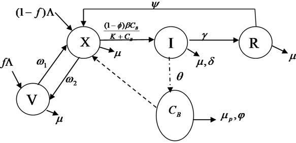
The transfer rates between the sub-classes are collection of several epidemiological parameters. The susceptible human population $(X)$ is increase by recruitment rate $Λ$ , the rate at which individuals is vaccinated is $ω_{2}$ and $f$ is the proportion of individuals who are vaccinated. The proportion of unvaccinated individuals is ( $1 - f$ ) and $ω_{1}$ is the rate of loosing immunity from vaccination individuals. $μ$ is the natural death rate which is applicable to all the classes. Bacteria $(C_{B})$ interact with $X$ and become infected with force of infection $β C_{B} / (K + C_{B})$ , it then move to infected class (I), where $β$ is the effective contact rate, also, K is the concentration of the bacteria in contaminated environment, and $C_{B} / (K + C_{B})$ is the probability of individuals in consuming foods or drinks contaminated caused by bacteria, the rate at which infected individuals die as a result of disease is $δ$ and $ϕ$ is the effectiveness of compliance of good hygiene. Meanwhile, The rate at which individuals recovered from $I$ class as a result of treatment from infection is $γ$ , there is no permanent recovery from the infection, recovery ( $R$ ) individuals move back to susceptible class at the rate of $ψ$ . Population of Bacteria $(C_{B})$ increase at the rate of $θ$ , the mortality rate of bacteria is $μ_{p}$ and the rate of sanitation which lead to death of bacteria is $φ$ . The model flow diagram is shown in Fig. 1. The dash line from Bacteria class $(C_{B})$ to susceptible class $(X)$ shows that susceptible individuals get the infection from Bacteria. The tick lines show the movement of one class to another class.

Based on the above schematic representation and assumptions of the models, the equations governing the dynamics of the Acute diarrhea infection are given as:

1

\frac{d X}{d t} = (1 - f) Λ + ω_{1} V + ψ R - \frac{β C_{B} (1 - ϕ)}{K + C_{B}} X - ω_{2} X - μ X,

2

\frac{d I}{d t} = \frac{β C_{B} (1 - ϕ)}{K + C_{B}} X - γ I - (μ + δ) I,

3

\frac{d V}{d t} = f Λ + ω_{2} X - ω_{1} V - μ V,

4

\frac{d R}{d t} = γ I - ψ R - μ R,

5

\frac{d C_{B}}{d t} = θ I - (μ_{p} + φ) C_{B},

6

N = X + I + V + R .

3. The model analysis

3.1. Invariant region

To obtain the invariant region, we considered the total human population ( $N$ ), where $N = X + I + V + R$ . Then, the differentiation of $N$ with respect to time leading to:

7

\frac{d N}{d t} = \frac{d X}{d t} + \frac{d I}{d t} + \frac{d V}{d t} + \frac{d R}{d t} .

Then we have:

8

N \leq \frac{Λ}{μ} - \{\frac{Λ - μ N_{0}}{μ}\} e^{- μ t} .

As $t \to \infty$ in Eq. (8), the population size $N \to Λ / μ$ which means that $0 \leq μ \leq Λ / μ$ . Thus, the feasible solution set of the system equations of the model enters and remains in the region: $Ω = {(X, I, V, R) \in R^{4} : N \leq Λ / μ}$ .

Therefore, the basic model is well posed epidemiologically and mathematically. Hence, it is sufficient to study the dynamics of the basic model in region $Ω$ .

3.2. The disease free equilibrium (DFE)

To find the disease free equilibrium, we set the Eq. (1) to zero (0) and solve simultaneously, we make $C_{B}$ in Eq. (6) subject of the expression and substitute into Eq. (2), we get:

9

I \{\frac{β X θ (1 - ϕ)}{K ((μ_{p} + φ) + θ I)} - γ - (μ + δ)\} = 0,

I = 0 o r \frac{β X θ (1 - ϕ)}{(K μ_{p} + K φ + θ I)} - γ - (μ + δ) = 0 .

Since $I = 0$ , then it implies $C_{B} = 0$ , $R = 0$ .Therefore, the disease free equilibrium:

10

E_{0} = (\frac{(1 - f) Λ (ω_{1} + μ) + f Λ ω_{1}}{(ω_{1} + μ) (ω_{2} + μ) - ω_{1} ω_{2}}, 0, \frac{f Λ μ + Λ ω_{2}}{(ω_{1} + μ) (ω_{2} + μ) - ω_{1} ω_{2}}, 0,0) .

3.3. The basic reproduction number $(R_{0})$

The $R_{0}$ is the secondary infection cases infected on average per person, to obtain the basic reproduction number, we used the next generation matrix which is the approach adopted by [3]. Both $F (x)$ and $V (x)$ are obtained from the model Eqs. (1-6) of the disease free equilibrium (DFE), we have:

I^{I} = \frac{β C_{B} (1 - ϕ) X}{K + C_{B}} - γ I - (μ + δ) I, C_{^{B}}^{I} = θ I - (μ_{p} + φ) C_{B} .

Therefore, $F (x)$ is the inflow of the infected class while $V (x)$ is the outflow of the infected class, we have the following:

f = (\begin{array}{l} f_{1} \\ f_{2} \end{array}) = (\begin{matrix} \frac{(1 - ϕ) β C_{B}}{K + C_{B}} X \\ θ I \end{matrix}), F = (\begin{array}{l} 0 & \frac{K (1 - ϕ) β}{(K + C_{B})^{2}} X \\ θ & 0 \end{array}) .

The Jacobian matrix of $f$ and $v$ evaluated at DFE are given by $F$ and $V$ , we get:

v = (\begin{matrix} (γ + μ + δ) I \\ (μ_{p} + φ) C_{B} \end{matrix}), V = (\begin{matrix} γ + μ + δ \\ 0 \end{matrix} \begin{matrix} 0 \\ μ_{p} + φ \end{matrix}) .

The characteristics equation of $F V^{- 1}$ is obtained with the inverse of $V$ as:

11

|(F V^{- 1}) - λ I| = (\begin{matrix} - λ & \frac{(1 - ϕ) β}{K (μ_{p} + φ)} X^{0} \\ \frac{θ}{γ + μ + δ} & - λ \end{matrix}) = 0 .

The dominant eigenvalues of $F V^{- 1}$ which is the spectral radius give:

12

λ = + \sqrt{\frac{θ}{(γ + μ + δ)} \frac{(1 - ϕ) β}{K (μ_{p} + φ)} X^{0}} .

Therefore, the basic reproduction number ( $R_{0}$ ) after substitution of $X^{0}$ is given as:

13

R_{0}^{2} = \frac{θ (1 - ϕ) β {(1 - f) Λ (ω_{1} + μ) + f Λ ω_{1}}}{(γ + μ + δ) K (μ_{p} + φ) {(ω_{1} + μ) (ω_{2} + μ) - ω_{1} ω_{2}}} .

3.4. Global stability of DFE

Theorem 1. The disease free equilibrium is globally asymptotically stable if $R_{0} < 1$ .

Proof: To show this theorem, we construct suitable Lyapunov function is given by:

14

L = θ I + (γ + μ + δ) C_{B} .

We differentiate Eq. (14) with respect to $t$ and substitute Eqs. (1-5) into the differentiation, we get:

15

\frac{d L}{d t} = θ \{\frac{β (1 - ϕ) C_{B} X}{K + C_{B}} - (γ + μ + δ) I\} + (γ + μ + δ) \{θ I - (μ_{p} + φ) C_{B}\} .

From Eq. (15) yields:

16

\frac{d L}{d t} = \frac{(γ + μ + δ) (μ_{p} + φ) K C_{B}}{K + C_{B}} \{R_{0}^{2} - \frac{(K + C_{B})}{K}\} .

So if $R_{0} < 1$ then $\frac{d L}{d t} < 1$ or if $C_{B} = 0 \Rightarrow \frac{d L}{d t} = 0$ . Hence, $L$ is Lyapunov function on $Ω$ and largest compact invariant set in ${(X, I, V, R, C_{B}) \in Ω, d L / d t = 0}$ is the singleton $(X, 0, V, 0,0)$ . Therefore, by Lasalle’s invariance principle Eq. (16), that all the solution of the model Eqs. (1-5) with initial condition in the region which approach the DFE at time tends to infinity when $R_{0} \leq 1$ , hence, DFE is globally asymptotically stable in the feasible region $Ω$ if $R_{0} \leq 1$ .

3.5. The endemic equilibrium

The endemic equilibrium state is denoted by $E^{*} = (X^{*}, I^{*}, V^{*}, R^{*}, {C_{B}}^{*})$ and this occurs when the infection is persistence in the population. To obtain this, we equate the system of Eqs. (1-5) to zero and we have the following:

17

E^{*} = (\frac{(γ + μ + δ) \{(μ_{p} + φ) K + θ I^{*}\}}{β (1 - ϕ) θ}, I^{*} > 0

\frac{f Λ β θ (1 - ϕ) + ω_{2} (γ + μ + δ) \{(μ_{p} + φ) K + θ I^{*}\}}{β θ (1 - ϕ) (ω_{1} + μ)}, \frac{γ I^{*}}{ψ + μ}, \frac{θ I^{*}}{μ_{p} + φ}) .

3.6. Global stability of endemic equilibrium (EE)

Theorem 2. If $R_{0} > 1$ , the endemic equilibrium state is globally asymptotically stable, otherwise, unstable if $R_{0} < 1$

Proof:

18

L = (X - X^{*} I n X) + (I - I^{*} I n I) + (C_{B} - {C_{B}}^{*} I n C_{B}) .

The differentiation of Eqs. (18) is gives by:

19

\frac{d L}{d t} = (1 - \frac{X^{*}}{X}) \frac{d X}{d t} + (1 - \frac{I^{*}}{I}) \frac{d I}{d t} + \frac{β (1 - ϕ) C_{B}^{*} X^{*}}{θ I^{*} (K + C_{B})} (1 - \frac{C_{B}^{*}}{C_{B}}) \frac{d C_{B}}{d t},

20

\frac{d L_{(X)}}{d t} = (1 - \frac{X^{*}}{X}) \{(1 - f) Λ + ω_{1} V + ψ R - \frac{β C_{B} (1 - ϕ) X}{(K + C_{B})} - ω_{2} X - μ X\} (1 - \frac{X^{*}}{X})

∙ \{- ω_{1} V^{*} - ψ R^{*} + \frac{β C_{B}^{*} (1 - ϕ) X^{*}}{(K + C_{B}^{*})} + ω_{2} X^{*} + μ X^{*} + ω_{1} V + ψ R - \frac{β C_{B} (1 - ϕ) X}{(K + C_{B})} - ω_{2} X - μ X\} (1 - \frac{X^{*}}{X}) \{\frac{β C_{B}^{*} (1 - ϕ) X^{*}}{(K + C_{B}^{*})} - \frac{β C_{B} (1 - ϕ) X}{(K + C_{B})} + ω_{2} X^{*} - ω_{2} X + μ X^{*} - μ X - ω_{1} V^{*} + ω_{1} V - ψ R^{*} + ψ R\} (1 - \frac{X^{*}}{X}) \{\frac{β C_{B}^{*} (1 - ϕ) X^{*}}{(K + C_{B}^{*})} - \frac{β C_{B} (1 - ϕ) X}{(K + C_{B})} + ω_{2} (X^{*} - X) + μ (X^{*} - X) - ω_{1} (V^{*} - V) - ψ (R^{*} - R)\} \frac{β C_{B}^{*} (1 - ϕ) X^{*}}{(K + C_{B}^{*})} (1 - \frac{X^{*}}{X})

∙ \{1 - \frac{X C_{B} (K + C_{B}^{*})}{X^{*} C_{B}^{*} (K + C_{B})}\} + (\frac{X - X^{*}}{X}) {(ω_{2} + μ) (X^{*} - X) - ω_{1} (V^{*} - V) - ψ (R^{*} - R)}

∙ \frac{β C_{B}^{*} (1 - ϕ) X^{*}}{(K + C_{B}^{*})} (1 - \frac{X^{*}}{X}) \{1 - \frac{X C_{B} (K + C_{B}^{*})}{X^{*} C_{B}^{*} (K + C_{B})}\} - \frac{(ω_{2} + μ)}{X} (X^{*} - X)^{2} - (\frac{X - X^{*}}{X}) {ω_{1} (V^{*} - V) + ψ (R^{*} - R)} \leq \frac{β C_{B}^{*} (1 - ϕ) X^{*}}{(K + C_{B}^{*})} (1 - \frac{X^{*}}{X}) \{1 - \frac{X C_{B} (K + {C_{B}}^{*})}{X^{*} C_{B}^{*} (K + C_{B})}\},

21

\frac{d L_{(I)}}{d t} = (1 - \frac{I^{*}}{I}) \frac{d I}{d t},

\frac{d L_{(I)}}{d t} = (1 - \frac{I^{*}}{I}) \{\frac{β C_{B} (1 - ϕ) X}{(K + C_{B})} - γ I - (μ + δ) I\},

\frac{d L_{(I)}}{d t} = (1 - \frac{I^{*}}{I}) \{\frac{β C_{B} (1 - ϕ) X}{(K + C_{B})} - \frac{β C_{B}^{*} (1 - ϕ) X^{*}}{(K + C_{B}^{*}) I^{*}} I\} = \frac{β (1 - ϕ) X^{*} C_{B}^{*}}{(K + C_{B}^{*})} (1 - \frac{I^{*}}{I}) \{\frac{\frac{X C_{B}}{(K + C_{B})}}{\frac{X^{*} C_{B}^{*}}{(K + C_{B}^{*})}} - \frac{I}{I^{*}}\},

22

\frac{d L_{(C_{B})}}{d t} = \frac{β (1 - ϕ) C_{B}^{*} X^{*}}{θ I^{*} (K + C_{B})} (1 - \frac{C_{B}^{*}}{C_{B}}) \frac{d C_{B}}{d t} = \frac{β (1 - ϕ) C_{B}^{*} X^{*}}{θ I^{*} (K + C_{B})} (1 - \frac{C_{B}^{*}}{C_{B}}) (θ I - (μ_{p} + φ) C_{B}),

\frac{d L_{(C_{B})}}{d t} = \frac{β (1 - ϕ) C_{B}^{*} X^{*}}{θ I^{*} (K + {C_{B}}^{*})} (1 - \frac{C_{B}^{*}}{C_{B}}) (θ I - \frac{θ I^{*} C_{B}}{C_{B}^{*}}) = \frac{β (1 - ϕ) C_{B}^{*} X^{*}}{(K + C_{B}^{*})} (1 - \frac{C_{B}^{*}}{C_{B}}) (\frac{I}{I^{*}} - \frac{C_{B}}{C_{B}^{*}}) .

As a result of Eqs. (20-22), we get:

23

\frac{d L}{d t} = \frac{d L_{(X)}}{d t} + \frac{d L_{(I)}}{d t} + \frac{d L_{(C_{B})}}{d t},

\frac{d L}{d t} \leq \frac{β C_{B}^{*} (1 - ϕ) X^{*}}{(K + C_{B}^{*})} (1 - \frac{X^{*}}{X}) \{1 - \frac{X C_{B} (K + C_{B}^{*})}{X^{*} C_{B}^{*} (K + C_{B})}\}

+ \frac{β (1 - ϕ) X^{*} C_{B}^{*}}{(K + C_{B}^{*})} (1 - \frac{I^{*}}{I}) \{\frac{\frac{X C_{B}}{(K + C_{B})}}{\frac{X^{*} C_{B}^{*}}{(K + C_{B}^{*})}} - \frac{I}{I^{*}}\} + \frac{β (1 - ϕ) C_{B}^{*} X^{*}}{(K + C_{B}^{*})} (1 - \frac{C_{B}^{*}}{C_{B}}) (\frac{I}{I^{*}} - \frac{C_{B}}{C_{B}^{*}}) .

For the function $V (X) = 1 - X + I n X$ , we know that $X > 0$ leads to $V (X) \leq 0$ and if $X = 1$ , then $V (X) = 0$ :

\frac{d L_{(X, I)}}{d t} \leq \frac{β C_{B}^{*} (1 - ϕ) X^{*}}{(K + C_{B}^{*})} (1 - \frac{X^{*}}{X}) \{1 - \frac{X C_{B} (K + C_{B}^{*})}{X^{*} C_{B}^{*} (K + C_{B})}\}

+ \frac{β (1 - ϕ) X^{*} C_{B}^{*}}{(K + C_{B}^{*})} (1 - \frac{I^{*}}{I}) \{\frac{\frac{X C_{B}}{(K + C_{B})}}{\frac{X^{*} C_{B}^{*}}{(K + C_{B}^{*})}} - \frac{I}{I^{*}}\},

24

\begin{array}{l} \frac{d L_{(X, I)}}{d t} \leq \frac{β C_{B}^{*} (1 - ϕ) X^{*}}{(K + C_{B}^{*})} (1 - \frac{X C_{B} (K + C_{B}^{*})}{X^{*} C_{B}^{*} (K + C_{B})} - \frac{X^{*}}{X} + \frac{C_{B} (K + C_{B}^{*})}{{C_{B}}^{*} (K + C_{B})}) \\ + \frac{β (1 - ϕ) X^{*} C_{B}^{*}}{(K + C_{B}^{*})} (\frac{\frac{X C_{B}}{(K + C_{B})}}{\frac{X^{*} C_{B}^{*}}{(K + C_{B}^{*})}} - \frac{I}{I^{*}} - \frac{\frac{X C_{B}}{(K + C_{B})}}{\frac{X^{*} C_{B}^{*}}{(K + C_{B}^{*})}} \frac{I^{*}}{I} + \frac{I^{*}}{I} \frac{I}{I^{*}}), \end{array}

\begin{array}{l} \frac{d L_{(X, I)}}{d t} \leq \frac{β C_{B}^{*} (1 - ϕ) X^{*}}{(K + C_{B}^{*})} (1 - \frac{X C_{B} (K + C_{B}^{*})}{X^{*} C_{B}^{*} (K + C_{B})} - \frac{X^{*}}{X} + \frac{C_{B} (K + C_{B}^{*})}{{C_{B}}^{*} (K + C_{B})}) \\ + \frac{β (1 - ϕ) X^{*} C_{B}^{*}}{(K + C_{B}^{*})} (\frac{X C_{B} (K + C_{B}^{*})}{X^{*} C_{B}^{*} (K + C_{B})} - \frac{I}{I^{*}} + \frac{I^{*} X C_{B} (K + C_{B}^{*})}{I X^{*} C_{B}^{*} (K + C_{B})} + 1), \end{array}

\frac{d L_{(X, I)}}{d t} \leq \frac{β C_{B}^{*} (1 - ϕ) X^{*}}{(K + C_{B}^{*})} (2 - \frac{X^{*}}{X} - \frac{I}{I^{*}} + \frac{C_{B} (K + C_{B}^{*})}{{C_{B}}^{*} (K + C_{B})} + \frac{I^{*} X C_{B} (K + C_{B}^{*})}{I X^{*} C_{B}^{*} (K + C_{B})}),

\frac{d L_{(X, I)}}{d t} \leq \frac{β (1 - ϕ) X^{*} C_{B}^{*}}{(K + C_{B}^{*})} (\frac{C_{B}}{C_{B}^{*}} - I n (\frac{C_{B}}{C_{B}^{*}}) - \frac{I}{I^{*}} + I n (\frac{I}{I^{*}})) .

Also:

25

\frac{d L_{(C_{B})}}{d t} = \frac{β (1 - ϕ) C_{B}^{*} X^{*}}{(K + C_{B}^{*})} (1 - \frac{C_{B}^{*}}{C_{B}}) (\frac{I}{I^{*}} - \frac{C_{B}}{C_{B}^{*}}) = \frac{β (1 - ϕ) C_{B}^{*} X^{*}}{(K + C_{B}^{*})} (\frac{I}{I^{*}} - \frac{C_{B}}{C_{B}^{*}} - \frac{C_{B}^{*}}{C_{B}} \frac{I}{I^{*}} + \frac{C_{B}}{C_{B}^{*}} \frac{C_{B}^{*}}{C_{B}}) \frac{d L_{(C_{B})}}{d t} = \frac{β (1 - ϕ) C_{B}^{*} X^{*}}{(K + C_{B}^{*})} (\frac{I}{I^{*}} - \frac{C_{B}}{C_{B}^{*}} - \frac{C_{B}^{*}}{C_{B}} \frac{I}{I^{*}} + 1) \frac{d L_{(C_{B})}}{d t} = \frac{β (1 - ϕ) C_{B}^{*} X^{*}}{(K + C_{B}^{*})} (v (\frac{C_{B}^{*}}{C_{B}} \frac{I}{I^{*}}) + \frac{I}{I^{*}} - I n (\frac{I}{I^{*}}) - \frac{C_{B}}{C_{B}^{*}} + I n (\frac{C_{B}}{C_{B}^{*}})),

\frac{d L_{(C_{B})}}{d t} \leq \frac{β (1 - ϕ) C_{B}^{*} X^{*}}{(K + C_{B}^{*})} (\frac{I}{I^{*}} - I n (\frac{I}{I^{*}}) - \frac{C_{B}}{C_{B}^{*}} + I n (\frac{C_{B}}{C_{B}^{*}})) .

Consequently, we have:

26

\frac{d L}{d t} \leq \frac{β (1 - ϕ) X^{*} C_{B}^{*}}{(K + C_{B} *)} (\frac{C_{B}}{C_{B}^{*}} - I n (\frac{C_{B}}{{C_{B}}^{*}}) - \frac{I}{I^{*}} + I n (\frac{I}{I^{*}})) + \frac{β (1 - ϕ) C_{B}^{*} X^{*}}{(K + C_{B}^{*})} (\frac{I}{I^{*}} - I n (\frac{I}{I^{*}}) - \frac{C_{B}}{C_{B}^{*}} + I n (\frac{C_{B}}{C_{B}^{*}})) \frac{d L}{d t} \leq \frac{β (1 - ϕ) X^{*} C_{B}^{*}}{(K + C_{B}^{*})} (\frac{C_{B}}{C_{B}^{*}} - I n (\frac{C_{B}}{C_{B}^{*}}) - \frac{I}{I^{*}} + I n (\frac{I}{I^{*}}) + \frac{I}{I^{*}} - I n (\frac{I}{I^{*}}) - \frac{C_{B}}{C_{B}^{*}} + I n (\frac{C_{B}}{C_{B}^{*}})),

\frac{d L}{d t} \leq \frac{β (1 - ϕ) X^{*} {C_{B}}^{*}}{(K + C_{B}^{*})} {0} = 0,

Implies:

27

\frac{d L}{d t} \leq 0 .

Therefore, it can be seen from Eqs. (27) that largest invariant subset when $d L / d t = 0$ is $E^{*}$ , by lasalle’s invariance principle, $E^{*}$ is globally asymptotically stable when $R_{0} > 1$ .

4. Extension of the model equations into optimal control system

The model of acute diarrhea infection is generalized by incorporating two control strategies. The control is $α_{1}$ which minimize the contact of susceptible and bacteria and control $α_{2}$ which is the treatment of individuals who developed symptoms of the infection. Therefore, incorporating the controls into the model, we get the following:

28

\frac{d X}{d t} = (1 - f) Λ + ω_{1} V + ψ R - (1 - α_{1}) (1 - ϕ) λ X - ω_{2} X - μ X,

29

\frac{d I}{d t} = (1 - α_{1}) (1 - ϕ) λ X - (α_{2} + γ) I - (μ + δ) I,

30

\frac{d V}{d t} = f Λ + ω_{2} X - ω_{1} V - μ V,

31

\frac{d R}{d t} = (α_{2} + γ) I - ψ R - μ R,

32

\frac{d C_{B}}{d t} = θ I - (μ_{p} + φ) C_{B},

where:

33

λ = \frac{C_{B} β}{K + C_{B}} .

Our main objective is to obtain the optimal levels of the controls and associated state variables that optimize the objective function. The objective functional is given by:

34

J (α_{1} (\cdot), α_{2} (\cdot)) = \int_{0}^{t_{f}} (b_{1} I + \frac{1}{2} \sum_{i = 1}^{2} {w_{i}}^{*} {α_{i}}^{2}) d t .

And the minimizing the cost function [2], that is $J ({α_{1}}^{*} (\cdot), {α_{2}}^{*} (\cdot)) = \underset{u_{1}, u_{2}}{m i n} (α_{1} (\cdot), α_{2} (\cdot))$ , where, $\{0 \leq α_{1} < 0.95,0 \leq α_{2} < 0.95\}$ , $\forall t \in [0, T]$ .

The state variable coefficients b and with controls $w_{1}$ , $w_{2}$ are positive. Since the cost is nonlinear in its condition, here we considered the cost with controls in a quadratic form $\frac{1}{2} {w_{i}}^{*} {α_{i}}^{2}$ [2]. The aim of this work is to minimize the number of infective and cost that is to get the optimal $(α_{1}^{*}, α_{2}^{*}) ∍ J (α_{1}^{*}, α_{2}^{*}) = m i n {(α_{1}, α_{2}) / α_{i} \in U}$ , where, $U = {(α_{1}, α_{2}) /$ each $α_{i}$ is measurable with $0 \leq α_{i} < 1$ for $0 \leq t \leq t_{f}}$ .

4.1. Existence of an optimal control

The Hamiltonian and Optimal system, we used the approach of [2] such that:

35

H = \frac{d J}{d t} + λ_{1} \frac{d X}{d t} + λ_{2} \frac{d I}{d t} + λ_{3} \frac{d V}{d t} + λ_{4} \frac{d R}{d t} + λ_{5} \frac{d C_{B}}{d t},

36

H (X, I, V, R, C_{B}) = L (X, I, V, R, C_{B}) + λ_{1} \frac{d X}{d t} + λ_{2} \frac{d I}{d t} + λ_{3} \frac{d V}{d t} + λ_{4} \frac{d R}{d t} + λ_{5} \frac{d C_{B}}{d t},

where, $L (X, I, V, R, C_{B}) = b I + \frac{1}{2} \sum_{i = 1}^{2} {w_{i}}^{*} {α_{i}}^{2}$ , $λ_{1}$ , $λ_{2}$ , $λ_{3}$ , $λ_{4}$ , and, $λ_{5}$ are the adjoint variable functions. To obtain the adjoint variables, we followed [2].

Theorem 3. There exist an optimal control $α_{1}$ and $α_{2}$ which are corresponding Solutions, $X$ , $I$ , $V$ , $R$ , and $C_{B}$ that minimize $J (α_{1}, α_{2})$ over $U$ there exist adjoint functions $λ_{1}$ , $λ_{2}$ , $λ_{3}$ , $λ_{4}$ , and, $λ_{5}$ :

37

\frac{d λ_{1}}{d t} = - λ_{1} (- (1 - α_{1}) \frac{β (1 - ϕ) C_{B}}{(K + C_{B})} - μ + ω_{2}) - λ_{2} ((1 - α_{1}) \frac{β (1 - ϕ) C_{B}}{(K + C_{B})}) - λ_{3} ω_{2},

38

\frac{d λ_{2}}{d t} = - b_{1} - λ_{2} (- α_{2} - γ - μ - δ) - λ_{4} (α_{2} + γ) - λ_{5} θ,

39

\frac{d λ_{3}}{d t} = - λ_{1} (ω_{1}) - λ_{3} (- ω_{1} - μ),

40

\frac{d λ_{4}}{d t} = - λ_{1} (ψ) - λ_{4} (- ψ - μ),

41

\frac{d λ_{5}}{d t} = - λ_{1} (- \frac{(1 - α_{1}) β (1 - ϕ) X}{(K + C_{B})} + \frac{(1 - α_{1}) β (1 - ϕ) C_{B} X}{(K + C_{B})^{2}})

- λ_{2} (\frac{(1 - α_{1}) β (1 - ϕ) X}{(K + C_{B})} - \frac{(1 - α_{1}) β (1 - ϕ) C_{B} X}{(K + C_{B})^{2}}) - λ_{5} (- μ_{p} - φ) .

With transverscility conditions, $λ_{i} (t_{f}) = 0$ , $i = 1, . . ., 5$ .

And the control of $(α_{1}^{*}, α_{2}^{*})$ is:

42

α_{1}^{*} (t) = m a x \{0, m i n (1, \frac{X (λ_{1} β C_{B} ϕ - λ_{2} β C_{B} ϕ)}{(K + C_{B}) w^{*}})\},

α_{2}^{*} (t) = m a x \{0, m i n (1, \frac{I (λ_{2} - λ_{4})}{w_{2}^{*}})\} .

Proof:

43

\frac{d λ_{1}}{d t} = - \frac{d H}{d X} = - λ_{1} (- (1 - α_{1}) \frac{β (1 - ϕ) C_{B}}{(K + C_{B})} - μ + ω_{2})

- λ_{2} ((1 - α_{1}) \frac{β (1 - ϕ) C_{B}}{(K + C_{B})}) - λ_{3} ω_{2},

\frac{d λ_{2}}{d t} = - \frac{d H}{d I} = - b_{1} - λ_{2} (- α_{2} - γ - μ - δ) - λ_{4} (α_{2} + γ) - λ_{5} θ,

44

\frac{d λ_{5}}{d t} = - \frac{d H}{d C_{B}} = - λ_{1} (- \frac{(1 - α_{1}) β (1 - ϕ) X}{(K + C_{B})} + \frac{(1 - α_{1}) β (1 - ϕ) C_{B} X}{(K + C_{B})^{2}})

- λ_{2} (\frac{(1 - α_{1}) β (1 - ϕ) X}{(K + C_{B})} - \frac{(1 - α_{1}) β (1 - ϕ) C_{B} X}{(K + C_{B})^{2}}) - λ_{5} (- μ_{p} - φ) .

And for characterisation of the optimal control, we used partial differential equations $\frac{\partial H}{d α_{i}} = 0$ , at $α_{i} = α_{i}^{*}$ , where, $i = 1,2$ .

For $i = 1$ , $\frac{\partial H}{\partial α_{1}} = 0$ at:

45

α_{1}^{*} = > α_{1}^{*} = \frac{X (λ_{1} β C_{B} ϕ - λ_{2} β C_{B} ϕ)}{(K + C_{B}) w_{1}^{*}} .

For $i = 2$ , $\frac{\partial H}{\partial α_{2}} = 0$ at:

46

α_{2}^{*} = > α_{2}^{*} = \frac{I (λ_{2} - λ_{4})}{w_{2}^{*}} .

Since $0 < α_{i}^{*} < 1$ , we can write in a compact notation:

47

α_{1}^{*} = m a x \{0, m i n (1, \frac{X (λ_{1} β C_{B} ϕ - λ_{2} β C_{B} ϕ)}{(K + C_{B}) w^{*}})\},

α_{2}^{*} = m a x \{0, m i n (1, \frac{I (λ_{2} - λ_{4})}{w_{2}^{*}})\} .

4.2. The optimality system

It is a system of Eqs. (28-32) and adjoint Eqs. (37-41) incorporating with the characteristics of optimal control and initial as well as transversality conditions. The following optimality is presented:

48

\frac{d X}{d t} = (1 - f) Λ + ω_{1} V + ψ R - (1 - α_{1}^{*}) (1 - ϕ) λ X - ω_{2} X - μ X,

49

\frac{d I}{d t} = (1 - α_{1}^{*}) (1 - ϕ) λ X - (α_{2}^{*} + γ) I - (μ + δ) I,

50

\frac{d V}{d t} = f Λ + ω_{2} X - ω_{1} V - μ V,

51

\frac{d R}{d t} = (α_{2}^{*} + γ) I - ψ R - μ R,

52

\frac{d C_{B}}{d t} = θ I - (μ_{p} + φ) C_{B},

53

\frac{d λ_{1}}{d t} = - λ_{1} (\frac{- (1 - α_{1}^{*}) β (1 - ϕ) C_{B}}{(K + C_{B})} - μ + ω_{2}) - λ_{2} (\frac{(1 - α_{1}^{*}) β (1 - ϕ) C_{B}}{(K + C_{B})}) - λ_{3} ω_{2},

54

\frac{d λ_{2}}{d t} = - b_{1} - λ_{2} (- α_{2}^{*} - γ - μ - δ) - λ_{4} (α_{2}^{*} + γ) - λ_{5} θ,

55

\frac{d λ_{3}}{d t} = - λ_{1} (ω_{1}) - λ_{3} (- ω_{1} - μ),

56

\frac{d λ_{4}}{d t} = - λ_{1} (ψ) - λ_{4} (- ψ - μ),

57

\frac{d λ_{5}}{d t} = - λ_{1} (- \frac{(1 - α_{1}^{*}) β (1 - ϕ) X}{(K + C_{B})} + \frac{(1 - α_{1}^{*}) β (1 - ϕ) C_{B} X}{(K + C_{B})^{2}})

- λ_{2} (\frac{(1 - α_{1}^{*}) β (1 - ϕ) X}{(K + C_{B})} - \frac{(1 - α_{1}^{*}) β (1 - ϕ) C_{B} X}{(K + C_{B})^{2}}) - λ_{5} (- μ_{p} - φ),

58

λ_{i} (t_{f}) = 0, i = 1,2, 3,4, 5, X (0) = X_{0}, I (0) = I_{0},

V (0) = V_{0}, R (0) = R_{0}, C_{B} (0) = C_{B_{0}}

5. Numerical results and discussion

The model is simulated using the parameter values in Table 1, to assess the effect of different strategies considered the two control measures in this study are education awareness, environmental sanitations and hygiene, and Treatment of an individuals. The graphical results obtained are shown below.

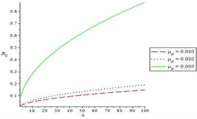
Fig. 2 shows the effect of compliance of good hygiene on basic reproduction number $R_{0}$ , it is observed from Fig. 1 that, as compliance rate of good hygiene ( $ϕ$ ) increases, the reproduction number decreases ( $R_{0}$ ). In Fig. 3, we varying the rate of effective contact rate ( $β$ ), we observed that as effective contact rate decreases, it also decreases the basic reproduction number. It is observed from Fig. 4 that as production rate of Bacteria infection $(θ)$ from infected human increases, it increases the basic reproduction number $R_{0}$ , varying the recovery rate ( $γ$ ), it was discovered that as recovery parameter increases, it decreases the basic reproduction number. Meanwhile, Fig. 5 shows the effect of recruitment rate ( $Λ$ ) on the basic reproduction number $R_{0}$ , it is observed that as recruitment rate ( $Λ$ ) increases, it increases the basic reproduction number $R_{0}$ .

Table 1Definition of the parameters and values

Symbol	Definition of the parameter	Value	Source
$Λ$	Human populations rate	100/day	[2]
$ω_{1}$	Rate of loosing immunity from vaccination individuals	0.55/day	Assumed
$ψ$	Rate of recovered humans to become Susceptible	0.003/day	[14]
$ω_{2}$	Rate at which individuals are vaccinated	0.45/day	Assumed
$β$	Exposure to contaminated food and water (Effective contact rate)	0.9/day	[2]
$ϕ$	Compliance rate of waters and foods Hygiene	0.6/days	Assumed
$γ$	Recovery rate of infected humans	0.002/day	[2]
$θ$	Production of Bacteria infection from infected humans	0.8cell/mL/day	Assumed
$μ$	Natural human mortality	0.0247/day	[2]
$δ$	Disease induced dearth rate	0.052/day	[2]
$f$	Proportion of unvaccinated individuals	0.075/day	Assumed
$K$	Concentration of the bacteria in contaminated water	50,000	[2]
$μ_{p}$	Mortality rate for bacteria	0.001/day	[2]
$φ$	Water Sanitation lead to dearth of Bacteria	0.05/day	Assumed

Fig. 2Effect of compliance of Hygiene on reproduction number

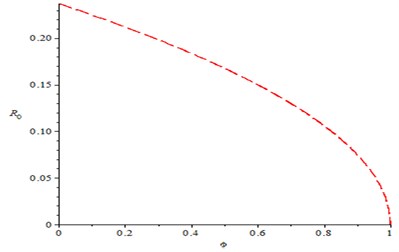
Fig. 3Varying the rate of exposure to contaminated foods and waters (β) on reproduction number

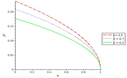
Fig. 4Production rate of Bacteria infection on reproduction number

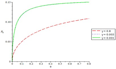
Fig. 5Effect of recruitment rate (Λ) on the basic reproduction number

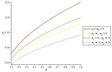
We examine the effect of $α_{1} (t)$ and $α_{2} (t)$ respectively, as two control measures ( $α_{1}$ , $α_{2}$ ) were used to optimize the objective function $J (α_{1} (\cdot), α_{2} (\cdot))$ . It means minimizing the contact between the infected and susceptible individuals, and treatment of acute diarrhea infectious is also optimized. We observed from Fig. 6, line one ( $α_{1} = α_{2} = 0$ ) that the acute diarrheal infection is not effectively control as basic reproduction number increases. In line two $(α_{1} = 0, α_{2} \neq 0)$ only $α_{2}$ is used to optimize the objective function $J (α_{1} (\cdot), α_{2} (\cdot))$ , while setting $α_{1}$ to zero, this is the only treatment without prevention and it is observed that it is not like having prevention by minimizing the contact between the infected individuals and susceptible. In line three ( $α_{1} \neq 0, α_{2} = 0$ ) with this measure, it is clearly suggested that this strategy is very efficient and effective in controlling the basic reproduction number of the model equations. In line four ( $α_{1} \neq α_{2} \neq 0$ ), we observed that acute diarrhea infection of individuals is effectively control as basic reproduction number reduces.

Fig. 6Effective contact rate on reproduction number, varying the control strategies

6. Conclusions

In this study, we presented an improved model for the transmission of acute diarrehea infection, two models were considered; we presented an acute diarrhea infection with effectiveness of compliance of good hygiene. The second model was an optimal control model that included two control measures with one minimizing the interaction between the susceptible and bacteria infectious, and the other is increasing the number of treated individuals. From the analysis, it was found that, the Disease Free Equilibrium is globally asymptotically stable if $R_{0} \leq 0$ and Endemic state is globally asymptotically stable when $R_{0} > 0$ . Graphically, the reproduction number shown significant reduction as the strategy ( $α_{1} \neq α_{2} \neq 0$ ) suggested that optimal prevention and treatment regime against acute diarrhea infection in a population would be a good approach to effectively control or eradicate the acute diarrhea infection.

References

Ochoa Blanca M. D., Surawicz Christina M. Diarrheal Diseases – Acute and Chronic, University of Washington School of Medicine, Seattle, 2002.

Search CrossRef
Tilahun G. T., Makinde O. D., Malonza D. Modelling and optimal control of typhoid fever disease with cost-effective strategies. Computational and Mathematical Method in Medicine, Vol. 2017, 2017, p. 2324518.

Publisher
Lasisi N. O., Akinwande N. I., Olayiwola R. O., et al. Mathematical model for Ebola virus infection in human with effectiveness of drug usage. Journal of Applied Sciences and Environmental Management, Vol. 22, Issue 7, 2018, p. 1089-1095.

Publisher
Bertoletti A., Maini M., Williams R. Role of hepatitis B virus specific cytotoxic T cells in liver damage and viral control. Antiviral Research, Vol. 60, Issue 2, 2003, p. 61-66.

Publisher
Abdulrahman S., Akinwande N. I., Awojoyogbe O. B., Abubakar U. Y. Sensitivity analysis of the parameters of A mathematics model of Hepatitis B virus transmissions. Universal Journal of Applied Mathematics, Vol. 1, Issue 4, 2013, p. 230-240.

Publisher
Akinwande N. I. A mathematical model of the dynamics of the HIV/AIDS disease pandemic. Journal of Nigeria Mathematical Society, Vol. 25, 2006, p. 99-108.

Search CrossRef
Culshaw Rebecca V., Shigui Ruan A delay-differential equation model of HIV infection of CD4+ T-cells. Journal of Mathematical Biosciences, Vol. 165, 2000, p. 27-39.

Publisher
Codecco C. T. Endemic and epidemic dynamics of cholera: the role of the aquatic reservoir. BMC Infection Disease, 2001, https://doi.org/10.1186/1471-2334-1-1.

Publisher
Pascual M., Bouma M. J., Dobson A. P. Cholera and climate: Revisiting the quatitative evidence. Microbes and Infection, Vol. 4, 2002, p. 237-245.

Publisher
Jensen M. A., Faruque S. M., Mekalanos J. J., Levin B. R. Modelling the role of bacteriophage in the control of Cholera outbreaks. Proceedings of the National Academy of Sciences of the United States of America, Vol. 103, Issue 12, 2006, p. 4652-4657.

Publisher
Tien J. H., Earn D. J. D. Multiple transmission pathways and disease dynamics in a waterborne pathogen mode. Bulletin of Mathematical Biology, Vol. 72, 2010, p. 1506-1533.

Publisher
Misra A. K., Singh V. A delay mathematical model for the spread and control of water borne diseases. Journal of Theoretical Biology, Vol. 301, 2012, p. 49-56.

Publisher
Lasisi N. O., Akinwande N. I., Oguntolu F. A. Development and exploration of a mathematical model for transmission of monkey-pox in humans. Journal of Mathematical Models in Engineering, Vol. 6, Issue 1, 2020, p. 23-33.

Publisher
Mwasa A., Tchuenche J. M. Mathematical analysis of a cholera model with public health interventions. Biosystems, Vol. 105, 2011, p. 190-200.

Publisher

Cited by

EFFECTS OF PUBLIC AWARENESS AND VACCINATION IN MODELING THE DYNAMICS OF MONKEY-POX TRANSMISSION DISEASE IN NIGERIA

Nurudeen Oluwasola Lasisi | Mohammed Rashad Abdullahi | Fahad Suleiman

(2024)

Modeling the effect of distancing and wearing of face masks on transmission of Covid-19 infection dynamics

Nurudeen O. Lasisi | Kolawole A. Adeyemo

(2021)

About this article

Received

05 April 2020

Accepted

31 May 2020

Published

30 June 2020

DOI

https://doi.org/10.21595/chs.2020.21409

Keywords

acute diarrhea infection

basic reproduction number

modelling

global stability

This is an open access article distributed under the Creative Commons Attribution License, which permits unrestricted use, distribution, and reproduction in any medium, provided the original work is properly cited.

Previous article in issue Previous Next article in issue Next

Research article

2024 02 18

Optimal control of autonomous vehicle path tracking based on whale optimization algorithm

Fang Han, Yingjie Liu, Wen Peng

Research article

2021 06 21

Lyapunov approach and global stability of Ebola virus infection model of an individual cells population

Nurudeen Oluwasola Lasisi

Research article

2021 06 11

Modeling the effect of distancing and wearing of face masks on transmission of Covid-19 infection dynamics

Nurudeen O. Lasisi, Kolawole A. Adeyemo

Research article

2020 11 05

Automated set-up parameter estimation and result evaluation for SSI-Cov-OMA

Lukas Bonekemper, Marcel Wiemann, Peter Kraemer

N. O. Lasisi, N. I. Akinwande, and S. Abdulrahaman, “Optimal control and effect of poor sanitation on modelling the acute diarrhea infection,” Journal of Complexity in Health Sciences, Vol. 3, No. 1, pp. 91–103, Jun. 2020, https://doi.org/10.21595/chs.2020.21409

Copy Extrica

Copied to clipboard!

TY  - JOUR
DO  - 10.21595/chs.2020.21409
UR  - https://doi.org/10.21595/chs.2020.21409
TI  - Optimal control and effect of poor sanitation on modelling the acute diarrhea infection
T2  - Journal of Complexity in Health Sciences
AU  - Lasisi, N. O.
AU  - Akinwande, N. I.
AU  - Abdulrahaman, S.
PY  - 2020
DA  - 2020/06/30
PB  - JVE International Ltd.
SP  - 91-103
IS  - 1
VL  - 3
SN  - 2538-7995
SN  - 2538-8002
ER  - 

Copy Ris

Copied to clipboard!

@article{Lasisi_2020,
	doi = {10.21595/chs.2020.21409},
	url = {https://doi.org/10.21595/chs.2020.21409},
	year = 2020,
	month = {jun},
	publisher = {{JVE} International Ltd.},
	volume = {3},
	number = {1},
	pages = {91--103},
	author = {N. O. Lasisi and N. I. Akinwande and S. Abdulrahaman},
	title = {Optimal control and effect of poor sanitation on modelling the acute diarrhea infection},
	journal = {Journal of Complexity in Health Sciences}
}

Copy Bibtex

Copied to clipboard!

[1]N. O. Lasisi, N. I. Akinwande, and S. Abdulrahaman, “Optimal control and effect of poor sanitation on modelling the acute diarrhea infection,” Journal of Complexity in Health Sciences, vol. 3, no. 1, pp. 91–103, Jun. 2020, doi: 10.21595/chs.2020.21409.

Copy IEEE

Copied to clipboard!

Lasisi, N. O., N. I. Akinwande, and S. Abdulrahaman. “Optimal Control and Effect of Poor Sanitation on Modelling the Acute Diarrhea Infection.” Journal of Complexity in Health Sciences 3, no. 1 (June 30, 2020): 91–103. https://doi.org/10.21595/chs.2020.21409.

Copy Chicago

Copied to clipboard!

Optimal control and effect of poor sanitation on modelling the acute diarrhea infection

Abstract

1. Introduction

2. Model formulation

3. The model analysis

3.1. Invariant region

3.2. The disease free equilibrium (DFE)

3.3. The basic reproduction number(R0)

3.4. Global stability of DFE

3.5. The endemic equilibrium

3.6. Global stability of endemic equilibrium (EE)

4. Extension of the model equations into optimal control system

4.1. Existence of an optimal control

4.2. The optimality system

5. Numerical results and discussion

6. Conclusions

References

Cited by

About this article

Related Articles

3.3. The basic reproduction number $(R_{0})$