Adomian’s decomposition method to modeling power functionally graded thermoelastic materials in heat transfer and thermal stress analysis

Youssef, Hamdy M.; Al-Lehaibi, Eman A. N.

doi:10.21595/vp.2019.20538

Vibroengineering Procedia

Browse Procedia

Published: 15 March 2019

Check for updates

Adomian’s decomposition method to modeling power functionally graded thermoelastic materials in heat transfer and thermal stress analysis

Hamdy M. Youssef¹

Eman A. N. Al-Lehaibi²

¹Mathematics Department, Faculty of Education, Alexandria University, Alexandria, Egypt

¹Mechanics Department, Faculty of Engineering, Umm Al-Qura University, Makka, Saudi Arabia

²Mathematics Department, Al-Lith University College, Umm Al-Qura University, Makka, Saudi Arabia

Corresponding Author:

Hamdy M. Youssef

Cite the article Download PDF

Downloads 1317

CrossRef Citations 1

0

Smart Citations

0

Citing PublicationsSupportingMentioningContrasting

View Citations

See how this article has been cited at scite.ai

scite shows how a scientific paper has been cited by providing the context of the citation, a classification describing whether it supports, mentions, or contrasts the cited claim, and a label indicating in which section the citation was made.

Abstract

This work deals with an iteration method for numerical solving the problem of one-dimensional coupled thermoelasticity under given boundary conditions. This iteration based on the Adomian’s decomposition method. All the material properties have been considered variable on position with a power law. The numerical results have been calculated for different cases of the gradient parameter and the gradient index. The numerical results have been shown in figures. The gradient parameter and the gradient index have significant effects on the temperature increment, the strain, the stress, and the displacement.

1. Introduction

Recently, much attention has been devoted to the numerical methods in which do not require discretization of time-space variables or to the linearization of the non-linear equations [1]. Adomian introduced the decomposition method for solving linear and non-linear ordinary and partial differential equations [2-4]. This method offers accurate and computable with approximately convergent solutions to linear and non-linear partial and ordinary differential equations [5-16]. Adomian got the solutions of many bio-mathematical models of viruses, bacteria, antigens, and tumor tissues [4]. Adomian’s decomposition method (ADM) is to divide the given equation into linear and nonlinear parts of the equation [1, 13].

2. Mathematical idealizations of a FGM by using power law

This particular idealization for FGM modeling is well-known in the fracture mechanics science. The thickness $h$ , the typical material properties $P (x)$ at any point at a distance $x$ from the reference surface has been modeled to this equation [17]:

1

$P (x) = P_{T o p} {(1 - R \frac{x}{h})}^{n}, R = (1 - \frac{P_{B o t}}{P_{T o p}}), P_{T o p} = {P (x)|}_{x = 0}, P_{B o t} = {P (x)|}_{x = L} .$

$R$ is the gradient parameter when it vanishes all the material properties are in the standard case with constant values. $n$ is the material gradient index which depends upon the design requirements [17].

3. Formulation the problem in general form

Consider an isotropic and thermo-elastic body in one-dimensional fill the region which is defined by $Ψ = \{x : 0 \leq x < h\}$ where $h$ is the thickness of the body, and it is initially at rest and has been loaded by the harmonic thermal wave, and the surface is traction free.

The displacement components for one-dimension medium have the form [18]:

2

$u (x, t) = u_{x} (x, t), u_{y} = u_{z} = 0 .$

The equation of motion:

3

$ρ (x) \frac{\partial^{2} e}{\partial t^{2}} = [λ (x) + 2 μ (x)] \frac{\partial^{2} e}{\partial x^{2}} - γ (x) \frac{\partial^{2} θ}{\partial x^{2}} .$

The generalized equation of heat conduction has the form:

4

$\frac{\partial}{\partial x} (K (x) \frac{\partial θ}{\partial x}) = ρ (x) C_{E} (x) \frac{\partial θ}{\partial t} + γ (x) T_{0} \frac{\partial e}{\partial t},$

5

$K (x) \frac{\partial^{2} θ}{\partial x^{2}} + \frac{\partial K (x)}{\partial x} (\frac{\partial θ}{\partial x}) = ρ (x) C_{E} (x) \frac{\partial θ}{\partial t} + γ (x) T_{0} \frac{\partial e}{\partial t} .$

The constitutive relation takes the form:

6

$σ = [λ (x) + 2 μ (x)] e - γ (x) θ, e = \frac{\partial u}{\partial x} .$

In the above equations, $θ = (T - T_{0})$ is the temperature increment, $ρ (x)$ is the density, $λ (x)$ and $μ (x)$ are Lame’s parameters, $K (x)$ is the thermal conductivity, $γ (x)$ is a material constant given by $γ (x) = [3 λ (x) + 2 μ (x)] α_{T} (x)$ , $α_{T} (x)$ being the coefficient of linear thermal expansion, and $C_{E} (x)$ is the specific heat at constant strain.

4. Formulation of the problem by using the exponential law

Substitute from Eq. (7) into Eqs. (4)-(6), we get:

7

$\{K (x), λ (x), μ (x), C_{E} (x), ρ (x), α_{T} (x)\} = \{K_{0}, λ_{0}, μ_{0}, C_{0 E}, ρ_{0}, α_{0 T}\} {(1 - R \frac{x}{h})}^{n},$

8

$ρ_{0} \frac{\partial^{2} e}{\partial t^{2}} = [λ_{0} + 2 μ_{0}] - γ_{0} {(1 - R \frac{x}{h})}^{n} \frac{\partial^{2} θ}{\partial x^{2}},$

9

${(1 - R \frac{x}{h})}^{n} \frac{\partial^{2} θ}{\partial x^{2}} - \frac{n R}{h} {(1 - R \frac{x}{h})}^{n - 1} (\frac{\partial θ}{\partial x}) = \frac{ρ_{0} C_{0 E}}{K_{0}} {(1 - R \frac{x}{h})}^{2 n} \frac{\partial θ}{\partial t}$

$+ \frac{γ_{0} T_{0}}{K_{0}} {(1 - R \frac{x}{h})}^{2 n} \frac{\partial e}{\partial t},$

10

$σ = (λ_{0} + 2 μ_{0}) {(1 - R \frac{x}{h})}^{n} e - γ_{0} {(1 - R \frac{x}{h})}^{2 n} θ .$

For simplicity, we use the non-dimensional variables (we will drop the primes) [18]:

11

$(x', u', h') = c_{0} η (x, u, h), t^{'} = c_{0}^{2} η t, θ^{'} = \frac{θ}{T_{0}}, σ = \frac{σ'}{(λ_{0} + 2 μ_{0})},$

where:

$η = \frac{ρ_{0} C_{0 E}}{K_{0}}, γ_{0} = (3 λ_{0} + 2 μ_{0}) α_{0 T}, c_{0} = \sqrt{\frac{λ_{0} + 2 μ_{0}}{ρ_{0}}}, ε_{1} = \frac{γ_{0} T_{0}}{λ_{0} + 2 μ_{0}}, ε_{2} = \frac{γ_{0}}{ρ_{0} C_{0 E}},$

thus, we obtain:

12

$\frac{\partial^{2} e}{\partial x^{2}} = \frac{\partial^{2} e}{\partial t^{2}} + ε_{1} {(1 - R \frac{x}{h})}^{n} \frac{\partial^{2} θ}{\partial x^{2}},$

13

$\frac{\partial^{2} θ}{\partial x^{2}} = {(1 - R \frac{x}{h})}^{n} \frac{\partial θ}{\partial t} + ε_{2} {(1 - R \frac{x}{h})}^{n} \frac{\partial e}{\partial t} + \frac{n R}{h} {(1 - R \frac{x}{h})}^{- 1} (\frac{\partial θ}{\partial x}),$

14

$σ = {(1 - R \frac{x}{h})}^{n} e - ε_{1} {(1 - R \frac{x}{h})}^{2 n} θ .$

Eq. (13) has been reduced to the form:

15

$\frac{\partial^{2} θ}{\partial x^{2}} = {(1 - R \frac{x}{h})}^{n} \frac{\partial θ}{\partial t} + ε_{2} {(1 - R \frac{x}{h})}^{n} \frac{\partial e}{\partial t} + \frac{n R}{h} (1 + R \frac{x}{h}) (\frac{\partial θ}{\partial x}) .$

5. Adomian’s decomposition method (ADM)

The differential operator $L$ is defined as following [8, 10, 15]:

16

$L_{x x} e (x, t) = L_{t t} e (x, t) + ε_{1} {(1 - R \frac{x}{h})}^{n} L_{x x} θ (x, t),$

17

$L_{x x} θ (x, t) = {(1 - R \frac{x}{h})}^{n} [L_{t} θ (x, t) + ε_{2} L_{t} e (x, t)] + \frac{n R}{h} (1 + R \frac{x}{h}) L_{x} θ (x, t) .$

The appeared operators in the above equations are defined as:

18

$L_{t} = \frac{\partial}{\partial t}, L_{t t} = \frac{\partial^{2}}{\partial t^{2}}, L_{x} = \frac{\partial}{\partial x}, L_{x x} = \frac{\partial^{2}}{\partial x^{2}} .$

Assuming that the inverse of the operator $L_{x}^{- 1}$ , $L_{x x}^{- 1}$ exists in the forms [8, 10, 15]:

19

$L_{x}^{- 1} f (x) = \int_{0}^{x} f (x_{1}) d x_{1}, L_{x x}^{- 1} f (x) = \int_{0}^{x} \int_{0}^{x_{2}} f (x_{1}) d x_{1} d x_{2} .$

Thus, applying the inverse operator on both the sides of Eqs. (17) and (18), we obtain:

20

$e (x, t) = e (0, t) + {\frac{\partial e (x, t)}{\partial x}|}_{x = 0} + L_{x x}^{- 1} [L_{t t} e (x, t) + ε_{1} {(1 - R \frac{x}{h})}^{n} L_{x x} θ (x, t)],$

21

$θ (x, t) = θ (0, t) + {\frac{\partial θ (x, t)}{\partial x}|}_{x = 0}$

$+ L_{x x}^{- 1} [{(1 - R \frac{x}{h})}^{n} L_{t} θ (x, t) + ε_{2} {(1 - R \frac{x}{h})}^{n} L_{t} e (x, t) + \frac{n R}{h} (1 + R \frac{x}{h}) L_{x} θ (x, t)] .$

We decompose the functions $θ (x, t)$ and $e (x, t)$ as following [8, 10, 15]:

22

$θ (x, t) = \sum_{k = 0}^{\infty} θ_{k} (x, t) = θ_{0} + \sum_{k = 1}^{\infty} θ_{k} (x, t), e (x, t) = \sum_{k = 0}^{\infty} e_{k} (x, t) = e_{0} + \sum_{k = 1}^{\infty} e_{k} (x, t),$

23

$e_{0} = e (0, t) + {\frac{\partial e (x, t)}{\partial x}|}_{x = 0}, θ_{0} = θ (0, t) + {\frac{\partial θ (x, t)}{\partial x}|}_{x = 0},$

24

$\sum_{k = 0}^{\infty} e_{k} (x, t) = e (0, t) + {\frac{\partial e (x, t)}{\partial x}|}_{x = 0}$

$+ L_{x x}^{- 1} [L_{t t} \sum_{k = 0}^{\infty} e_{k} (x, t) + ε_{1} {(1 - R \frac{x}{h})}^{n} L_{x x} \sum_{k = 0}^{\infty} θ_{k} (x, t)],$

25

$\sum_{k = 0}^{\infty} θ_{k} (x, t) = θ (0, t) + {\frac{\partial θ (x, t)}{\partial x}|}_{x = 0}$

$+ L_{x x}^{- 1} [\begin{array}{l} {(1 - R \frac{x}{h})}^{n} L_{t} \sum_{k = 0}^{\infty} θ_{k} (x, t) + ε_{2} {(1 - R \frac{x}{h})}^{n} L_{t} \sum_{k = 0}^{\infty} e_{k} (x, t) \\ + \frac{n R}{h} (1 + R \frac{x}{h}) L_{x} \sum_{k = 0}^{\infty} θ_{k} (x, t) \end{array}] .$

We obtain these components by $e_{k} (x, t)$ and $θ_{k} (x, t)$ the recursive formulas [8, 10, 15]:

26

$e_{k + 1} (x, t) = L_{x x}^{- 1} [L_{t t} e_{k} (x, t) + ε_{1} {(1 - R \frac{x}{h})}^{n} L_{x x} θ_{k} (x, t)], k \geq 1,$

27

$θ_{k + 1} (x, t) = L_{x x}^{- 1} {(1 - R \frac{x}{h})}^{n} [L_{t} θ_{k} (x, t) + ε_{2} L_{t} e_{k} (x, t)]$

$+ \frac{n R}{h} L_{x x}^{- 1} (1 + R \frac{x}{h}) L_{x} θ_{k} (x, t), k \geq 1 .$

The bounding plane $x =$ 0 is thermally loaded by harmonic heat and traction free as follows:

28

${θ (x, t)|}_{x = 0} = θ^{0} s i n (ω t), {\frac{\partial θ (x, t)}{\partial x}|}_{x = 0} = 0, {σ (x, t)|}_{x = 0} = 0, {\frac{\partial e (x, t)}{\partial x}|}_{x = 0} = 0 .$

Moreover, the series solutions of Eq. (22) are convergent very rapidly in real physical problems as in [12, 13]. The convergence of the series has investigated by several authors in [1, 5, 8, 9, 12-15]. In an algorithmic form, the suitable value for the tolerance $T o l =$ 10^-6 [10]:

6. The numerical results

The constants of the material properties were taken as follows [18]: $K_{0} =$ 386 W/(mK), $α_{0 T} =$ 1.78×10-5K^-1, $C_{0 E} =$ 383.1 J/(kgK), $η =$ 8886.73 s/m², $T_{0} =$ 293 K, $μ_{0} =$ 3.86×1010 N/m², $λ_{0} =$ 7.76×10¹⁰ N/m², $ρ_{0} =$ 8954 kg/m³, $ε_{1} =$ 0.0104443, $ε_{2} =$ 1.60862, $ω = π$ , $θ^{0} =$ 1.0, $h =$ 1.0.

Fig. 1θx,2.0 distribution for R= 0.0, 0.1

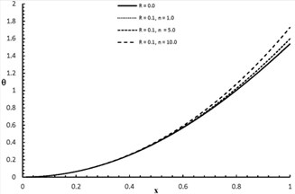
Fig. 2ex,2.0 distribution when R= 0.0, 0.1

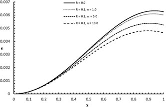
Fig. 3σx,2.0 distribution when R= 0.0, 0.1

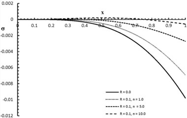
Fig. 4ux,2.0 distribution when R= 0.0, 0.1

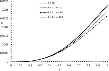
Fig. 5θx,2.0 distribution when R= 0.0, 0.5

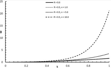
Fig. 6ex,2.0 distribution when R= 0.0, 0.5

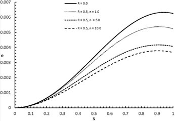
Fig. 7σx,2.0 distribution when R= 0.0, 0.5

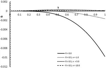
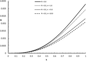
Fig. 8ux,2.0 distribution when R= 0.0, 0.5

7. Conclusions

Figs. 1-8 represent the temperature increment, the strain, the stress, and the displacement distribution with various values of the gradient parameter. $R =$ 0.0 gives the normal case of non-functionally graded material, while $R \neq 0.0$ performs a functionally graded material of power law with different values $R =$ (0.1, 0.2). From the consideration in Eq. (1), $R =$ 0.1 means that the ratio $P_{B o t} =$ 90 % $P_{T o p}$ , and $R =$ 0.2 gives that the ratio $P_{B o t} =$ 80 % $P_{T o p}$ . According to the results and the figures, the parameter $R$ has significant effects on all the stat-functions $θ = θ (x, t)$ , $e = e (x, t)$ , $σ = σ_{x x} (x, t)$ , and $u = u (x, t)$ . Moreover, $n$ has been assumed with different values through the calculations ( $n =$ 1, 5, 10) which give various materials’ designs. Figs. 1, 3, 5 and 7 show that when the value of the parameters $n$ and $R$ increase, the value of the temperature increment and the absolute value of the stress increase, while Figs. 2, 4, 6, and 8 show that when the value of the parameters $n$ and $R$ increases the value of the strain and the displacement decrease.

References

Sweilam N. Harmonic wave generation in non linear thermoelasticity by variational iteration method and Adomian’s method. Journal of Computational and Applied Mathematics, Vol. 207, Issue 1, 2007, p. 64-72.

Publisher
Adomian G. Solving Frontier Problems of Physics: The Decomposition Method. Klumer, Boston, 1994.

Publisher
Adomian G. Nonlinear Stochastic Systems Theory and Applications to Physics. Springer Science and Business Media, 1988.

Publisher
Adomian G., Cherruault Y., Abbaoui K. A nonperturbative analytical solution of immune response with time-delays and possible generalization. Mathematical and Computer Modelling, Vol. 24, Issue 10, 1996, p. 89-96.

Publisher
Ciarlet P., Jamelot E., Kpadonou F. Domain decomposition methods for the diffusion equation with low-regularity solution. Computers and Mathematics with Applications, Vol. 74, Issues 10, 2017, p. 2369-2384.

Publisher
Duz M. Solutions of complex equations with Adomian decomposition method. TWMS Journal of Applied and Engineering Mathematics, Vol. 7, Issue 1, 2017, p. 66-73.

Search CrossRef
El-Sayed S.-M., Kaya D. On the numerical solution of the system of two-dimensional Burgers’ equations by the decomposition method. Applied Mathematics and Computation, Vol. 158, Issue 1, 2004, p. 101-109.

Publisher
Górecki H., Zaczyk M. Decomposition method and its application to the extremal problems. Archives of Control Sciences, Vol. 26, Issue 1, 2016, p. 49-67.

Publisher
Kaya D., El-Sayed S.-M. On the solution of the coupled Schrödinger-KdV equation by the decomposition method. Physics Letters A, Vol. 313, Issue 1, 2003, p. 82-88.

Publisher
Kaya D., Inan I. E. A convergence analysis of the ADM and an application. Applied Mathematics and Computation, Vol. 161, Issue 3, 2005, p. 1015-1025.

Publisher
Kaya D., Yokus A. A decomposition method for finding solitary and periodic solutions for a coupled higher-dimensional Burgers equations. Applied Mathematics and Computation, Vol. 164, Issue 3, 2005, p. 857-864.

Publisher
Lesnic D. Convergence of Adomian’s decomposition method: periodic temperatures. Computers and Mathematics with Applications, Vol. 44, Issues 1-2, 2002, p. 13-24.

Publisher
Lesnic D. Decomposition methods for non-linear, non-characteristic Cauchy heat problems. Communications in Nonlinear Science and Numerical Simulation, Vol. 10, Issue 6, 2005, p. 581-596.

Publisher
Li L., Jiao L., Stolkin R., Liu F. Mixed second order partial derivatives decomposition method for large scale optimization. Applied Soft Computing, Vol. 61, 2017, p. 1013-1021.

Publisher
Mustafa I. Decomposition method for solving parabolic equations in finite domains. Journal of Zhejiang University-Science A, Vol. 6, Issue 10, 2005, p. 1058-1064.

Publisher
Vadasz P., Olek S. Convergence and accuracy of Adomian’s decomposition method for the solution of Lorenz equations. International Journal of Heat and Mass Transfer, Vol. 43, Issue 10, 2000, p. 1715-1734.

Publisher
Toudehdehghan A., Lim J., Foo K. E., Ma’arof M., Mathews J. A brief review of functionally graded materials. MATEC Web Conferences: EDP Sciences, 2017.

Publisher
Youssef H. M., El-Bary A.-A. Thermoelastic material response due to laser pulse heating in context of four theorems of thermoelasticity. Journal of Thermal Stresses, Vol. 37, Issue 12, 2014, p. 1379-1389.

Publisher

Cited by

Power law modeling of functionally graded Adomian’s decomposition method for thermoelastic materials in heat transfer and thermal stress analysis

Eman A. N. Al-Lehaibi

(2024)

About this article

Received

21 January 2019

Accepted

28 January 2019

Published

15 March 2019

SUBJECTS

Mathematical models in engineering

DOI

https://doi.org/10.21595/vp.2019.20538

Keywords

Adomian’s decomposition method

thermoelasticity

iteration method

power law

functionally graded

This is an open access article distributed under the Creative Commons Attribution License, which permits unrestricted use, distribution, and reproduction in any medium, provided the original work is properly cited.

Previous article in issue Previous Next article in issue Next

Research article

2023 12 23

Plane waves in an isotropic thermoelastic diffusive material using strain gradient theory

Baljeet Singh, Himanshu Singla

Research article

2023 06 26

Influence of the fractional-order strain on an infinite material with a spherical cavity under Green-Naghdi hyperbolic two-temperature thermoelasticity theory

Hamdy M. Youssef, Abdulrahman A. Alghamdi

Research article

2021 11 11

Influence of laser pulse on plane waves propagating in a thermoelastic medium with micro-temperature under the DPL model

Adnan Jahangir, Adiya Dar, Mohamed I. A. Othman

Research article

2021 09 13

Hyperbolic two-temperature generalized thermoelasticity with fractional order strain of solid cylinder

Alaa A. El-Bary

H. M. Youssef and E. A. N. Al-Lehaibi, “Adomian’s decomposition method to modeling power functionally graded thermoelastic materials in heat transfer and thermal stress analysis,” Vibroengineering PROCEDIA, Vol. 22, pp. 188–193, Mar. 2019, https://doi.org/10.21595/vp.2019.20538

Copy Extrica

Copied to clipboard!

TY  - JOUR
DO  - 10.21595/vp.2019.20538
UR  - https://doi.org/10.21595/vp.2019.20538
TI  - Adomian’s decomposition method to modeling power functionally graded thermoelastic materials in heat transfer and thermal stress analysis
T2  - Vibroengineering PROCEDIA
AU  - Youssef, Hamdy M.
AU  - Al-Lehaibi, Eman A. N.
PY  - 2019
DA  - 2019/03/15
PB  - JVE International Ltd.
SP  - 188-193
VL  - 22
SN  - 2345-0533
SN  - 2538-8479
ER  - 

Copy Ris

Copied to clipboard!

@article{Youssef_2019,
	doi = {10.21595/vp.2019.20538},
	url = {https://doi.org/10.21595/vp.2019.20538},
	year = 2019,
	month = {mar},
	publisher = {{JVE} International Ltd.},
	volume = {22},
	pages = {188--193},
	author = {Hamdy M. Youssef and Eman A. N. Al-Lehaibi},
	title = {Adomian's decomposition method to modeling power functionally graded thermoelastic materials in heat transfer and thermal stress analysis},
	journal = {Vibroengineering {PROCEDIA}}
}

Copy Bibtex

Copied to clipboard!

[1]H. M. Youssef and E. A. N. Al-Lehaibi, “Adomian’s decomposition method to modeling power functionally graded thermoelastic materials in heat transfer and thermal stress analysis,” Vibroengineering PROCEDIA, vol. 22, pp. 188–193, Mar. 2019, doi: 10.21595/vp.2019.20538.

Copy IEEE

Copied to clipboard!

Youssef, Hamdy M., and Eman A. N. Al-Lehaibi. “Adomian’s Decomposition Method to Modeling Power Functionally Graded Thermoelastic Materials in Heat Transfer and Thermal Stress Analysis.” Vibroengineering PROCEDIA 22 (March 15, 2019): 188–93. https://doi.org/10.21595/vp.2019.20538.

Copy Chicago

Copied to clipboard!

Adomian’s decomposition method to modeling power functionally graded thermoelastic materials in heat transfer and thermal stress analysis

Abstract

1. Introduction

2. Mathematical idealizations of a FGM by using power law

3. Formulation the problem in general form

4. Formulation of the problem by using the exponential law

5. Adomian’s decomposition method (ADM)

6. The numerical results

7. Conclusions

References

Cited by

About this article

Related Articles