Kernel PCA in nonlinear visualization of a healthy and a faulty planetary gearbox data

1. Introduction

The aim of this paper is to show a real (non-simulated) example illustrating how powerful and how easy are the classic and the kernel PCA for using in monitoring or diagnosing aspects of data analysis. The classic Principal Component Analysis (PCA) is very popular multivariate method dealing with feature extraction and dimensionality reduction [1]. It is based on sound mathematical algorithms inspired by geometrical concepts. It permits to extract from multi-dimensional data (MD-data) new meaningful features, mutually orthogonal. See in [2, 3] effective examples of applications to gearbox data.

Yet, in some obvious cases, the PCA may fail in recognizing the data structure. There is the famous example with two classes of 2D data points representing a ring and its center [4]. PCA is here useless; it is not able to visualize the data. Yet, to get the proper structure of these data, it is sufficient to add to the 2-dimensional data ($x,y$) a 3-rd dimension by defining a 3-rd variable $z=x^2+y^2$. Then, in the 3-dimensional space ($x,y,z$), the two classes appear perfectly separable.

Thus, the question: Could linearly inseparable data be transformed into some linearly separable ones? The answer is yes, it is sometimes possible, only one has to find the proper transformation. The kernel methodology proved to be helpful here.

In the following we will consider the kernel PCA [4]. This is a methodology which extends (transforms) the observed variables to a (usually) larger set of new derived variables constituting a new feature space $\mathcal{F}$. The extended features express the non-linear higher order relations between the observed variables (like in the ring and center example mentioned above). More features means more information on the data. So, carrying out the classical PCA in the extended space we expect more meaningful results. The computational algorithm retains the simplicity of the classic PCA computations [1] where the goal is clearly set and the optimization problem reduces to solving an eigen-problem for a symmetric matrix of Gram type.

A big number of derived new features might cause here some problems with time of computation and memory demands. A good deal of these problems can be solved efficiently by using the two paradigms:

1. The useful for us solutions yielded by PCA carried out in the extended feature space may be formulated in terms of inner products of the transformed variables (how to do it: see e.g., [5]).

2. One may use for the extension so called Mercer’s kernels $k\left(\mathbf{x},\mathbf{y}\right)$, and apply to them so called ’kernel trick’ (see [5]), which allows to obtain the results of kPCA using only input data to classic PCA.

Combining the two paradigms, one comes to the amazing statement that kernel PCA – with all its benefits – may be computed by using only the data vectors from the observed input data space, without making physically the extensions (transformations).

Our goal is to show, how the kernel PCA works for some real gearbox data. The acquisition and meaning of the data is described in [6], see also [2]. Generally, the data are composed from two sets: B (basic, healthy) and A (abnormal, faulty) gathered as vibration signals during work of a healthy and a faulty gearbox. The vibration signals were cut into segments; each segment was subjected to spectral (Fourier) analysis, yielding $d=\text{15}$ PSD variables memorized as a real vector $x=(x_1,\dots ,x_d{)}^T\in R^d$. In the following we will analyze a part of the data from [6]. The B set contains 500 data vectors, from these 439 gathered under normal load, and 61 – under small or no load of the first gearbox. The A set contains also 500 data vectors, from these 434 gathered under normal load, and 66 - under small or no load of the second gearbox being in abnormal state. Thus, the analysed data contain four meaningful subgroups. Our main goal is providing graphical visualization of the data. Will the 4-subgroup structure be recognisable from a (k)PCA analysis?

Our present analysis is set differently as in [2] under the three following aspects: 1. Learning methodology. Set B will be considered as the training data set, and the set A as the test data set. 2. Subgroup content. Both groups have a finer structure, indicating for heavy or small load of the gearboxes. 3. An additional method, the Kernel PCA will be used for analysis.

In the following, Section 2 describes shortly the principles of the classic PCA and its extended version: the kernel PCA (kPCA). Section 3 contains our main contribution: evaluation and visualization of the first three principal components expressed in the coordinate system constructed from the training data set. Section 4 contains Discussion and Closing Remarks.

2. Classic and kernel principal component

Generally, Principal Component Analysis (PCA) proceeds in three basic steps:

• Step 1. Computing covariance matrix $\mathbf{C}$ from a centered data matrix for the healthy gearbox taken as training data set.

• Step 2. Computing eigenvectors of $\mathbf{C}$, that is solving for $v$ the equation $\mathbf{C}\mathbf{v}=\mathbf{\lambda }\mathbf{v}$.

• Step 3. Projection of data points/data vectors using the eigenvectors obtained in step 2.

The computations in step 1 and step 2 are carried out using the training set of the data. The formula derived in step 3 shows how to compute projections for data vectors ${\mathbf{x}}_i$ belonging to the training data B. The same formula is valid for any data vector $\mathbf{x}$ residing in $R^d$, however under the condition, that this data vector is centered similarly as the data vectors ${\mathbf{x}}_i\in B$ (that is using means from B).

The idea of kernel PCA is to perform a nonlinear mapping $\mathrm{\Phi }$ of the input space $R^d$ to an extended feature space $\mathcal{F}$ and perform there the classical linear PCA. The mapping function is usually denoted as $\mathrm{\Phi }$ and that of individual data vectors/data points $\mathbf{x}$ as $\varphi$:

The positive fact of extending the number of features is that now these features may capture the internal structure of the data more accurately. The unfavorable aspects may be that the computing will need more time and memory, and may become unfeasible. Happily, we can get around this problem and still get the benefit of high-dimensional data. The classical PCA algorithm can be reformulated by expressing the necessary calculations in $\mathcal{F}$ as inner products (dot products), that may be obtained as specific kernel functions evaluated from the input vectors in $R^d$. This approach is called ’the kernel trick’ [4, 5, 7].

To perform kPCA one should know two important notations: that of the dot product and that of a kernel function. The dot product for two vectors $\mathbf{x}$ and $\mathbf{y}$ belonging to the same space $R^d$ denotes the inner product between these vectors:

Considering the mapped data vectors $\varphi \left(\mathbf{x}\right)$ and $\varphi \left(\mathbf{y}\right)$ in the feature space $\mathcal{F}$, their dot product in the feature space is defined as:

provided that we know explicitly how to evaluate the function $\varphi (.)$ in $\mathcal{F}$, and want to compute the needed dot product implicitly that way.

Alternatively, the needed dot product may be obtained via the kernel trick from a kernel function $k(\mathbf{x},\mathbf{y})$ with the property, that for all $\mathbf{x}$ and $\mathbf{y}$ belonging to the observed space $R^d$ one computes a kind of similarity measure between the pair $(\mathbf{x},\mathbf{y})$ yielding the value just equal to the inner product of the non-linearly transformed data vectors $\mathbf{x}$ and $\mathbf{y}$ living (after the transformation) in an extended data space $\mathcal{F}$ as $\varphi \left(\mathbf{x}\right)$ and $\varphi \left(\mathbf{y}\right)$. This may be summarized in the equation:

The exact form of the transformation is here not relevant, because one needs for the analysis only the values of the dot products, which are obtained by evaluating the kernel elements $k(\mathbf{x},\mathbf{y})$ without using in them explicite the $\varphi (.)$ function.

For a data set composed from $n$ data vectors ${\mathbf{x}}_i$, $i=1,\dots ,n$, one obtains the size $n\times n$ kernel matrix $\mathbf{K}$ as $\mathbf{K}=\left\{k\right({\mathbf{x}}_i,{\mathbf{x}}_j\left)\right\}$, $i$, $j=1,\dots ,n.$ Kernels widely used in data analysis are:

$•$ rbf (Gaussian) kernels: $k(x,y)=\mathrm{e}\mathrm{x}\mathrm{p}(\mathrm{}-\mathrm{}||\mathbf{x}-\mathbf{y}|{|}^2/c)$, with $c$ denoting a constant called kernel width;

$•$ polynomial kernels: $k(\mathbf{x},\mathbf{y})=(\mathbf{x}\cdot \mathbf{y}{)}^p$, for some positive $p$ denoting the degree of the polynomial. In the following we will use the rbf (Gaussian) kernels computed as:

where $\mathbf{d}=\mathbf{x}-\mathbf{y}$, and the kernel width parameter $c>0$ is found by trial and error.

When computing the kPCA we realize the three steps of classic PCA listed above, however with some modifications when using the kernel trick approach. For details, see [4].

Now let’s go to computing the PCA for our data.

3. Results of PCA and kPCA for the gearbox data

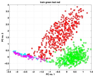
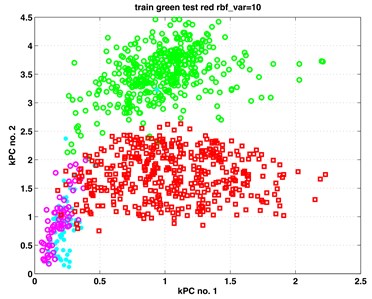
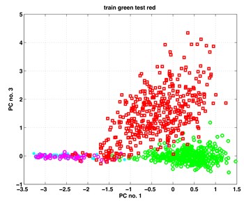
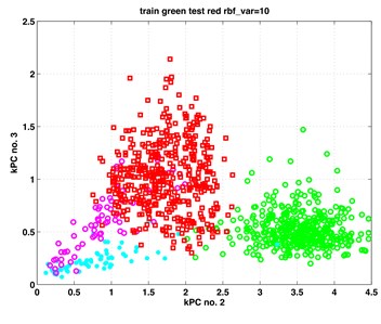
In this section, we present our results from the analysis of the gearbox data when applying to them the classic and kernel PCA. For both methods, the first three principal components (PCs) proved to contain relevant information on the subgroup structure of the data. In Fig. 1 we show scatterplots of the pairs (PC1, PC2), (PC1, PC3) – obtained by classic PCA, and scatterplots of pairs (kPC1, kPC2), (kPC2, kPC3) as containing the most relevant information. The exhibits in left column of Fig. 1 are results of classic PCA, and those in the right column – of kernel PCA.

The data points in the scatterplots represent time instances of the recorded vibrations. It is essential to inspect the exhibits in colour. There are four colours representing four subgroups of the analysed data. Data points from set B (healthy, work with full load) are painted in green. Those from set B (healthy, work with small or no load) are painted in cyan. Analogously, data points from set A (faulty, full load) are painted in red; those from set A (faulty, small or no load) are painted in magenta colour.

The set B served here as the basic training set for evaluation of the coordinate system capturing the main directions of the data cloud B. The analysis was performed using basic data standardized to have 0 means. The test data A were standardized using the means from the training group B.

Looking at the scatterplots in Fig. 1, one discerns there in all exhibits two big clouds of green and red data points corresponding to the fully loaded state of the gearboxes. The shapes of the clouds are near to ellipsoidal. Both clouds are not fully disjoint; they have few points covering common area. The read points have a larger scatter. This may be notified in all exhibits of the figure.

The two small subgroups with the magenta and cyan data points behave differently when using the two methods. In the PCA exhibits they appear as one undistinguishable set attached to the big red data cloud. Kernel PCA shows them also attached to the red data cloud, however in a rather distinguishable manner.

We may summarize out results that both PCA and kPCA yield equally good results concerning the healthy and faulty data, yet kPCA yields more details concerning the details of the structure of the data.

Our results were obtained using a modified code of Scholkopf’s toy_example.m available, for example, at: http://www.kernel-machines.org/code/kpca_toy.m.

Fig. 1Scatterplots of four pairs of principal components

a) Classic PCA, (PC1, PC2)

b) Kernel PCA, (kPC1, kPC2)

c) Classic PCA, (PC1, PC3),

d) Kernel PCA, (kPC2, kPC3)

4. Discussion and final results

We have analyzed two groups of data obtained from acoustic vibration signals from two different gearboxes: a healthy and a faulty one. Each of the groups contained a larger sub-group of instances gathered under normal load of the machine, and a much smaller sub-group gathered under small or no load of the machine. Usually the instances under small or no load are omitted from the analysis, because they may constitute a factor confusing the proper diagnosis. However, we took them to our analysis.

Using classic PCA and kernel PCA we extracted from the data a small number of meaningful principal components (PCs) and visualized them pairwise in scatterplots shown in Fig. 1. The PCs in that figure are shown in the coordinate system obtained from the eigenvectors of the healthy data set.

One may see in Fig. 1 that the big red and green data points (indicating full load) are distinguishable and practically linearly separable (with very few exceptions). This happens both for results from classic and kernel PCA. However, the smaller groups of magenta and cyan points (under-loading) are in the left exhibits overlapping; while in the right exhibits they are distinguishable, especially in the right bottom exhibit. Thus, the kernel PCA yielded here more information about the structure of the investigated data.

This kind of analysis opens immediately the way to diagnostics of the gearbox system with respect to its healthy or faulty functioning. It is possible to continue the analysis using some more sophisticated methods like in [8], permitting to find the kind of the fault. In any case, the main answer about state of the device, can be easily perceived from the simple scatterplots of few kernel PCs.

To this end we would like to emphasize, that our goal was just visualize the data in a plane to see what’s going on. To perform formally such tasks like discriminant analysis or clustering of the data, obviously one should use special methods dedicated to these tasks (see, for example, [9]). Our goal was just to visualize the data for getting directions of further research – following the motto Data with Insight Leads you to Decisions with Clarity launched by NYU STERN MS in Business Analytics.