Abstract
In order to monitor, analyze and diagnose the conditions of all kinds of machines, it is often necessary to calculate the probability density function of the sampled vibration signal. A new direct calculation method of probability density from sampled vibration signal based on the linear interpolation method (LIM) is presented in this paper. Two advantages are observed: 1) the time length of each amplitude segment obtained from a sampled vibration signal by the LIM is closer to the original continuous vibration signal, and 2) the calculation results of probability density got by calculating directly the ratio of time length of each amplitude segment to the total time of sampled vibration signal are more correct than those obtained by other existing methods. The applications to sampled simulation and actual vibration signals of a rolling bearing show that the probability density curves obtained by the new direct calculation method are more accurate and smoother than the curves got by other estimating methods used in a lot of famous software.
1. Introduction
There is abundant information in a sampled vibration signal. The probability density function of a vibration signal reflects the probability that the signal takes different amplitude. Different vibration signals have different shapes of probability density curves [1]. Some fault feature information is related to the probability density function of a vibration signal. Through analyzing the probability density function, the running condition of a device may be assessed, and fault features may be found.
At present, many researchers studied the algorithms of probability density function and its applications. Zhang [2] studied seven kernel functions, calculated the optimal bandwidth of different kernel functions, and pointed out that the Epanechnikov kernel function and the Quartic kernel function have the best estimation effect. Li [3] proposed an algorithm for blind source separation based on the estimation of probability density, which can be used to all the blind source separation algorithms where the score function is obtained by a nonlinear function. Zhao [4] proposed a recursive detection algorithm for the probabilities of random phase signals, which have the infinite series. Using the least squares and maximum likelihood estimator (MLE), Zhi [5] fit a signal with noise through the least squares moving algorithms, got a group of data with noise and did the MLE. The estimation of a signal gradually approaches the exact value, what provided an effective method for signal de-noising. Sha et al. [6] and Xu et al. [7] checked the normality and the amplitude distribution of a vibration signal using probability density functions.
Song et al. [8] put forward a method of intelligent condition diagnosis of rotating machinery using the probability density analysis and the canonical discriminant analysis, diagnosed the faults of a centrifugal blower. By combining the statistics of filter and probability density functions, Song et al. [9] proposed a novel fault diagnosis method and diagnosed the faults of gears on the experimental device. After empirical mode decomposition (EMD), Grasso et al. [10] put forward a novel criterion to assess the dissimilarity between adjacent CMFs based on probability density functions of frequency spectra. Boškoski et al. [11] made use of information indices based on the Rényi entropy derived from coefficients of the wavelet packet transform from measured vibration records and probability density of the envelope from a sum of sinusoidal signals with random amplitude and phase and proposed a novel approach for the diagnosis of a two-stage gearbox. Szolc et al. [12] proposed several stochastic methods for detection and identification of cracks in the shafts of rotating machines based on special probability density functions for crack locations and depths. Dimentberg [13, 14] studied a two-degree-of-freedom model which accounts for the non-linearity in external or “non-rotating” damping. He got an explicit expression for a stationary joint probability density of displacements and velocities as an exact analytical solution to the corresponding Fokker-Planck-Kolmogorov equation, which is used to detect the instability of the operating shaft. He analyzed a single mass/two-degrees-of-freedom rotating shaft with internal linear or “rotating” damping and external nonlinear damping with transverse vibrations. He obtained an analytical solution of the probability density of squared radius of the shaft whirl, and detected in on-line shaft instability. Zhuang et al. [15] presented a time-domain analysis method based on the probability density estimation for rotating machine fault detection. The probability density estimation based on the Parzen window was introduced. By inspecting the change of the probability density of a vibration signal, the machine condition was monitored.
From the above studies, we know that the probability density function is very useful in signal processing and fault diagnosis, such as the amplitude distribution of a vibration signal can be analyzed, and morphological detection of a vibration signal can be done by using the probability density function [6, 7]; the faults can be diagnosed by combining the probability density analysis with fault feature extraction and pattern recognition methods [8-15], and so on. Therefore, it is very important to calculate the probability density function of a vibration signal accurately. Although there are some functions in MATLAB [16, 17] and LabVIEW [18] to calculate the probability density, the accuracy of probability density curve is affected by the ratio between the number of sampling points and the size of segments in the histogram estimation because of the limitations of their calculation principles and by the window function type, window width, and number of sampling points and so on in the Parzen window density estimation. So, it is very important to study a more accurate calculation method of getting the probability density function.
A direct calculation method of probability density from a sampled vibration signal based on the linear interpolation method (LIM) is provided. This method contributes to that both the time length of each amplitude segment obtained from a sampled vibration signal by the LIM is closer to the original continuous vibration signal, and to that the calculation results of probability density got by calculating directly the ratio of time length of each amplitude segment to the total time of sampled vibration signal are more correct than those obtained by other existing methods. The applications to sampled simulation and actual vibration signals of a rolling bearing show that the probability density curves obtained by the new direct calculation method are more accurate and smoother than the curves got by other estimating methods used in a lot of famous software.
2. Definition of probability density function
2.1. Original definition of probability density function
2.1.1. Distribution function
Let is a random variable, is any real number, is a random event, corresponding to which there is a definite probability , the following function is called as the distribution function of :
For any two real numbers, , (), there is:
So, the distribution function represents the probability that falls on [, ]. The statistical laws of random variables are described completely by its distribution function.
2.1.2. Definition of probability density function
If there is a nonnegative integral function , for any real number there is [19]:
is called as the probability density function for .
If is continuous at point , then :
2.2. Definition of signal probability density function
The probability of the amplitude of a signal represents the chance or probability of instantaneous amplitude of a dynamic signal. The probability density of the signal amplitude is the probability within a unit amplitude segment, which is a function of its amplitude [20, 21].
A set of straight lines parallel to the abscissa are drawn, the distance between each other is on its waveform, as shown in Fig. 1. The probability which amplitude of the signal falls between and is determined by , where is the total signal observation time, is the time which amplitude is in [, ] of the total time, that is . If is infinite, the ratio will approach more accurately the event probability as follows:
For a sampling time sequence , 0, 1, 2, …, , the definition is expressed as:
where, is the sampling numbers; is the total number of amplitudes located in [, ].
Fig. 1Definition of signal probability density
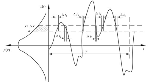
When the distance is infinitely small, the probability density of signal amplitude is as follows:
For a sampling time sequence , we have:
2.3. Probability density function of sinusoidal signal
The expression of a sinusoidal signal and its probability density function are as follows:
where, is the amplitude of the sinusoidal signal.
In Eq. (9), let 10, 20, 0, the sinusoidal signal is expressed as Eq. (11). Its waveform, probability density curve and probability distribution are shown in Fig. 2:
Fig. 2The waveform, probability density and distributions of a sinusoidal signal
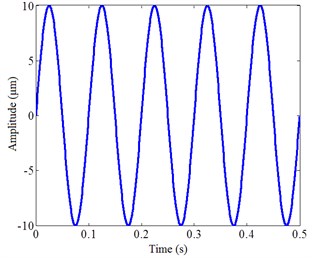
a) Waveform
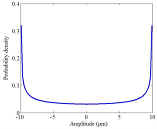
b) Probability density
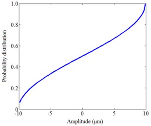
c) Probability distribution
3. Methods for probability density estimation
There are two basic methods for the probability density estimation: parametric estimation and nonparametric estimation. Parametric estimation is that the probability density function form of each class is known, and its parameters are unknown, but they will be estimated according to the samples. The common methods for parametric estimation are maximum likelihood estimation, Bayesian estimation and so on. The nonparametric estimation is that the class type of a sample is known, its probability density function form is unknown, but it is not directly by estimating the density function, including the function form and relevant parameters. The common methods for nonparametric estimation are histogram estimation, Rosenblatt estimation, Parzen window density estimation (kernal density estimation), nearest neighbor estimation and so on. Because the distributions types of the data sample for a vibration signal collecting from a rolling bearing are unknown, the nonparametric estimation method is commonly used to calculate its probability density by MATLAB and LabVIEW.
4. Problems of probability density calculation by common software
For a vibration signal, the data samples are some discrete data points with a certain sampling frequency. The probability density of a discrete signal is usually applied as the ratio of the total number of points falling into a certain segment to the number of the data points of the entire signal instead of the corresponding time. Although this substitution could be used to draw the probability density curve of the signal, the accuracy of the results will be affected by the sample sizes and the number of the segments being divided. Because the probability density curve of a typical signal is known, the sinusoidal signal shown in Eq. (11) is taken as an example to find the problems in its probability density calculation.
4.1. Problems of calculating probability density by MATLAB
There are two functions used in the nonparametric estimation in MATLAB. The function ksdensity is mainly used to analyze the continued distribution of a data sample, which is not adapted to calculate the probability density of rolling bearings. The hist function is a kind of function in MATLAB to do Histogram estimation, which is used to display the distribution of a data set. Another nonparametric estimation, the Parzen window density estimation may be used to calculate the probability density of a signal by its programming in MATLAB.
4.1.1. Probability density calculation by the hist function
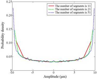
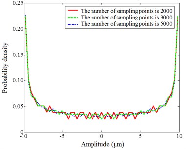
When calculating the probability density with the hist function for a vibration signal, the results are the data points distributed in each segment, which is called as a frequency number. In order to observe the calculation results easily, the probability is got by the frequency number in each segment ratio to the total signal sampling points. The sinusoidal signal is taken as an example, the number of sampling points and that of segments is changed, and the hist function is used, the probability density curves are got, as shown in Fig. 3.
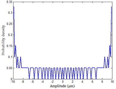
Fig. 3 shows that the basic shape of the probability density curve is correct when it is got directly by the hist function in MATLAB, and it is a concave curve. When the number of sampling points is 5000, and the number of divided segments is increased from 11 to 51, three kinds of probability density curves are basically smooth at both ends. However, with the increase of the number of divided segments, the middle of the curve turns to injustice, even with the appearance of some small serrates. When the number of sampling segments is kept 51, and the number of sampling points is changed, the middle part of the probability density curve is also uneven, and the less the number of sampling points is, the more fluctuated the middle part will be. This shows that the ratio between the numbers of sampling points and the segments should be set rationally when using the hist function. Otherwise the unideal results will be got. Fig.4 shows the amplified result of the unmatched ratio between the number of sampling numbers and the segments. It means that, when the number of sampling points of a sinusoidal signal is 1000, the segments are 101, the volatility of the probability density curve is quite severe, and the amplitude density of some segments is even zero.
Fig. 3Probability density of the sinusoidal signal calculated by the hist function in different parameters
a) Number of sampling points is 5000
b) Number of segments is 51
In Fig. 3 and Fig. 4, the probability density curve fluctuates that is because the number of data dispersed in different amplitude segments is calculated with the hist function by statics respectively. When two adjacent points are crossed in more than one amplitude segments, the time between two points should be distributed over each amplitude segment, but the actual calculation only takes the statistics in the segment where two data points are located, the time in the middle of each segment is totally ignored. When the neglecting effects are gradually increased, their occurrence probability in some segments will be shown in Fig. 4. That is, the number of sampling points is small, and the number of segments is large, which leads to that there are no data points in some partial amplitude segments, so the probability density will be 0.
Fig. 4Probability density of the sinusoidal signal calculated by the hist function when the number of sampling points is 1000 and that of segments is 101
4.1.2. Probability density calculation by Parzen window density estimation
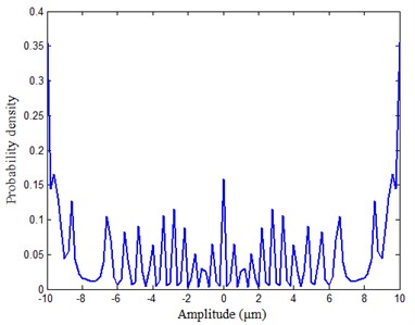
The Parzen window density estimation, which is also called as the kernel density estimation, is a kind of nonparametric estimation method. Firstly, the hypercube is established around the sample point. And then the appropriate window function is selected to find the number of samples falling into the hypercube. At last, the probability density curve is got by using the probability density formula. However, the number of samples and window width will have effects on the probability density curve. If the window width is too small, there may be no samples in some areas; if it is too large, the estimation curves will be flat, what will not reflect the overall distribution [22].
The probability density curves of the sinusoidal shown in Eq. (11) calculated by the Parzen window density estimation with different window functions, window width and the number of sampling points are shown in Fig. 5.
In Fig. 5(a) and Fig. 5(b), the exponential window function and normal window function are used in estimating the probability density respectively, the number of sampling points is 1000, and the window width is 1. Two probability density curves both fluctuate greatly. There are larger differences between two curves at both ends of the curves. In Fig. 5(b) and Fig. 5(c), the normal window function is used, and the window width is 1. When the number of sampling points is different, the curve fluctuation is improved as the number of sampling points increases. In Fig. 5(b) and Fig. 5(d), the normal window function is used; the number of sampling points is 1000. The fluctuation in Fig. 5(d) with the window width is 4 is lighter than that in Fig. 5(b) with the window width is 1, but there are sudden inflections in two sides of the curves shown in Fig. 5(d).
The above analysis shows that the results by Parzen window density estimation method are affected by the window function, window width, and number of sampling points and so on.
Fig. 5Probability density of the sinusoidal signal calculated by the Parzen window density estimation in different parameters
a) Number of sampling points is 1000, window width is 1, exponential window function is used
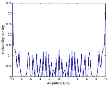
b) Number of sampling points is 1000, window width is 1, normal window function is used
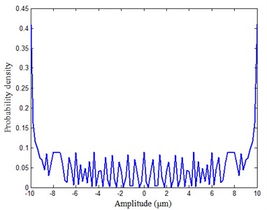
c) Number of sampling points is 2000, window width is 1, normal window function is used
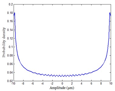
d) Number of sampling points is 1000, window width is 4, normal window function is used
4.2. Problems of calculating probability density by LabVIEW
In LabVIEW, there are also methods for calculating the probability density of a vibration signal. The calculation diagram is shown in Fig. 6. The sinusoidal signal shown in Eq. (11) is produced by the simulation signal generator in LabVIEW, which is put into Histogram.vi. The numbers of samples, segments and the smoothing numbers are set before calculation. The histogram estimation is used to calculate the probability density. Then the probability density and probability distribution of a sinusoidal signal are output. The corresponding probability density curves with different parameters are shown in Fig. 7.
Fig. 6Calculation diagram of probability density in LabVIEW
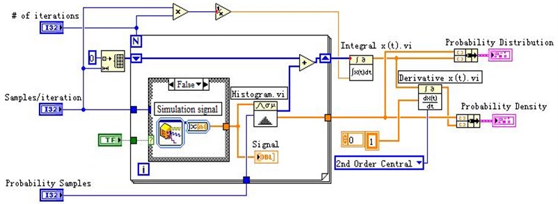
Fig. 7Probability density curves with different parameters in LabVIEW
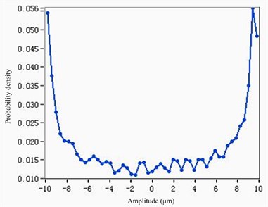
a) Number of sampling points is 1000, and that of segments is 51
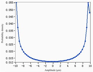
b) Number of sampling points is 1000, and that of segments is 51 with 10 times on average
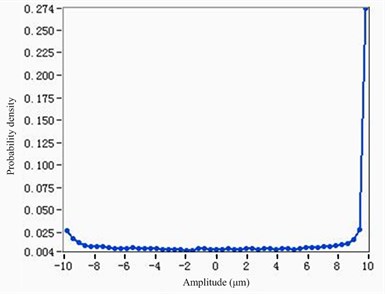
c) Number of sampling points is 2000, and that of segments is 51
When the number of sampling points is 1000, and the number of divided segments is 51, the middle of the probability density curve is fluctuating, what is similar to the result from MATLAB. In addition, there is a sudden inflection point at the far right of the curve in Fig. 7(a). The reason is that the time of the middle amplitude segment is ignored when the data point statistics method is used. The fluctuations in the probability density curve weaken after setting the average times in LabVIEW, what is better than that in MATLAB, shown in Fig. 7(b). The probability density curve becomes smoother when the average times are changed from 1 to 10 with other parameters unchanged, but the far right side of the inflection point problem in the curve is still unable to be solved. If the number of sample points is increased to 2000, the problems in the right most inflection points will be solved, but that will lead to a partial loss of the probability density curve, as shown in Fig. 7(c).
5. A direct calculation method of probability density from a sampled vibration signal based on LIM
From the fourth section, we know that the hist function in MATLAB and the method used in LabVIEW are all the histogram estimation methods. The results calculated by them are affected by the ratio between the number of sampling points and the size of the segments because of the limitations of their calculation principles. There will be some errors in probability density curves such as fluctuating, inflection points, 0 value of probability density, some lost parts of curve, and so on. And there are also errors in probability density curves got by the Parzen window density estimation, because they will be affected by the type of window function, window width, and number of sampling points and so on.
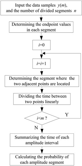
In order to solve the above problems, a direct calculation method of probability density from a sampled vibration signal based on LIM is proposed. In this method, the time ratio is used to approximate the probability of a certain segment in accordance with the original definition. The method is that, first, two adjacent data points are examined from the first data point of a vibration signal, and the segments, where the data points are located, are determined. Then the time between two points is divided into all the segments based on the LIM to prevent from no time distribution in any segment. This method is repeated until the last two points of the signal are counted. At last, the times of each amplitude segment are summed respectively, as shown in Fig. 8.
1) Getting the range of each segment of the samples according to the divided segments.
The divided segments of a sample are . The minimum and maximum values of the sampled data are the endpoint values of the total segments, which are equally divided into aliquots. The values of endpoints in each segment can be determined in turn, and then they can be recorded in the array , as there are 1 elements altogether.
2) Dividing the time between each adjacent data points.
First, the segment position, where two adjacent data points are located, will be determined. Suppose that there are sampling points in the given data, which is recorded in the array , and determine the segments where the first and second sampling points and are located as an example.
A loop is set, each endpoints element in of each segment is subtracted from in turn, such as , , then the product of is checked. If the product is negative or zero, the point is in this segment, the cycle will be ended. If the product is positive, the same method is used to calculate the product of the next segment until the product is not greater than zero. Similarly, the segment of the second sampling point can be determined.
After the segment of two adjacent points located in is determined, the time between two points will be divided. Let and is in the and segment, the time from to will be divided into three parts, shown in Fig. 9. That is, is in the segment, is in the segment, , ,…, are the time in the segments between the and segments. Among them, the calculation methods of time in and segments are the same, the calculation methods of time are as follows.
The sampling points and are connected with a line, the slope of the line is calculated, that is:
where, and are the time corresponding to the first and the second sampling points respectively.
And then, the time of the segment according to the slope is got, among which, 0 shows that two points are in the same segment. The time between two points is included into the segment. When 0, there are two cases of , positive and negative, the calculating methods are different, as shown in Fig. 10.
Fig. 8Process of the new calculation method for probability density
If is positive:
If is negative:
is assigned to , then the same method is used to get . At last, the time in every segment between and segment is got by average:
3) Calculating the total time.
For each adjacent sampling point, the calculations will be done according to step (2), and the time of each segment is recorded in the same column in each calculation, and the matrix is obtained after all the calculations are complete, is the division segments, and is the number of the sampling points. The matrices are summed by rows, the total time to of each segment is obtained.
4) Calculating the approximate probability:
where, is the time segment between adjacent data points.
5) Calculating the probability density of each segment:
Fig. 9Time divisions between two adjacent points
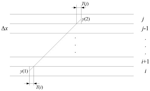
Fig. 10Calculation of Δt when k≠ 0
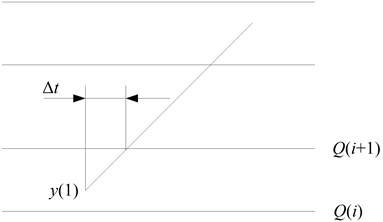
a) 0
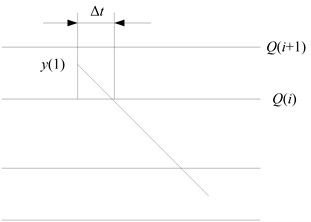
b) 0
6. Program and results analysis
The direct calculation method of probability density from a sampled vibration signal based on the LIM by MATLAB is used in the following calculations. The parameters are the same as those in 4.1 by MATLAB and 4.2 by LabVIEW. For the problems that the curve fluctuation, and the probability of the hist function is 0 in partial segments, the sampling points are still set to 1000, and the segments are set to 101 with the same sinusoidal signal, the corresponding result is shown in Fig. 11(a). For the problems of the inflection points and partial curves missing in LabVIEW, the segments are still 51, and sampling points are set to 1000 and 2000, the probability density is shown in Fig. 11(b) and Fig. 11(c).
Fig. 11 shows that in the new method, with the same parameters, the probability density curve is symmetrical and concave, all the parts of the curve are smooth basically, and the problem of zero probability density due to more segments and less sampling points is solved. In addition, for the same sinusoidal signal, the segments are unchanged, the number of sampling points is changed, the results are basically the same. And there are no sudden inflection points on the right end and no missing curves after increasing the sampling points that demonstrates that the new method is more accurate.
Fig. 11Probability density of the sinusoidal signal calculated by new method
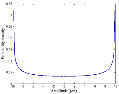
a) Number of sampling points is 1000 and that of segments is 101
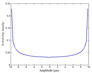
b) Number of sampling points is 1000 and that of segments is 51
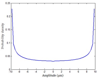
c) Number of sampling points is 2000 and that of segments is 51
7. Application and discussion
A sampled vibration signal is more complex than a sinusoidal signal. In order to verify the superiority of the direct calculation method of probability density from sampled vibration signal based on the LIM, four kinds of vibration signals collected from the test stand provided by the rolling bearing data center in the Case Western Reserve University of America are used [23]. The bearing data sets are widely used by researchers to analyze vibration signals of rolling bearings and their faults [24-26]. There is a motor, torque encoder, dynamometer and set of control electronics in the test stand, shown in Fig. 12. The vibration signals are collected by accelerometers. Four kinds of vibration signals are collected from deep groove ball bearing SKF6205 at the drive end, including normal running condition, inner raceway faults, and outer raceway faults and rolling element faults, single point faults were introduced to the test bearings using electro-discharge machining, the parameters are shown in Table 1.
Fig. 12Rolling bearing test stand
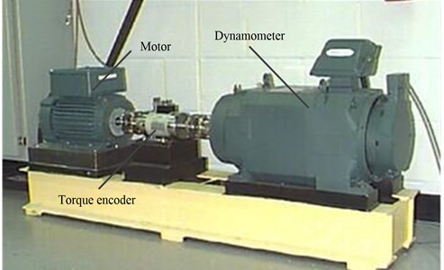
Table 1Testing parameters
No. | Item | Value | Unit |
1 | Rotating speed | 1797 | r/min |
2 | Sampling frequency | 12 | kHz |
3 | Number of sampling points | 2048 | – |
4 | Fault diameter | 0.18 | mm |
5 | Load of rolling bearing | 0 | – |
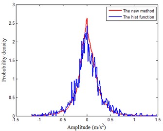
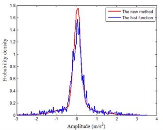
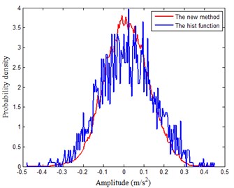
The waveforms of 4 kinds of vibration signals are shown in Fig. 13. When the probability density is calculated with the hist function and new method, the number of segments is 200, the results are shown in Fig. 14. A comparison of the time spent in calculating the probability density of four kinds of vibration signals from rolling bearing by the two methods are listed in Table 2. The calculating time is got by MATLAB R2012a on Windows 7 operation system in ThinkPad X200 which CPU is Intel Core 2 Duo P8400 with 2.26 GHz frequency and 6 GB memory.
Table 2Comparison of the time spent in calculating the probability density by the two methods
Working conditions | By the new method (s) | By the hist function (s) |
Normal running condition | 0.454155 | 1.069608 |
Inner raceway faults | 0.436880 | 1.052565 |
Outer raceway faults | 0.466030 | 1.307899 |
Rolling element faults | 0.603929 | 1.132706 |
From Fig. 14, we see that for four vibration signals from rolling bearing, the trends of the probability density curves calculated by the hist function and the method proposed in this paper are coincident, but those curves obtained by the new method have fewer fluctuations than those curves got by the hist function. And Table 2 shows that the time spent in calculating the probability density by the new method is faster than that by the hist founction.
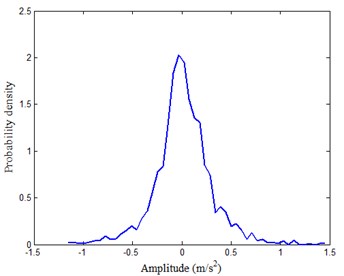
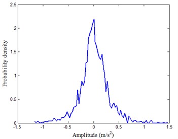
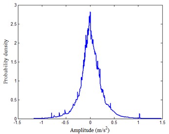
In order to further analyze and verify the influence of the number of segments on the probability density curve with two methods, the number of divided segments is set to 50, 100 or 1000 respectively for the inner raceway faults of the rolling bearing, and the probability density curves are shown in Fig. 15 and Fig. 16.
It can be seen from Fig. 15 that for the same vibration signals, there are fewer fluctuations in the probability density curves got by the hist function when the segments are less, and the curve fluctuations are becoming more and more when the segments increase, especially when the segments are 1000, the fluctuations are quite serious.
Fig. 16 shows that the probability density curves of the same signals have fewer fluctuations than those in Fig. 15 and the influence of the segment numbers is very small by using the new method. That demonstrates that the new method is more accurate than the existing method whether it is used in a simple sinusoidal signal or complex vibration signal.
Fig. 13Waveform of different vibration signal
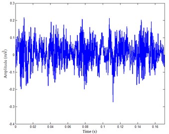
a) Normal running condition
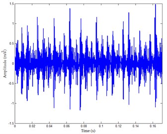
b) Inner raceway faults
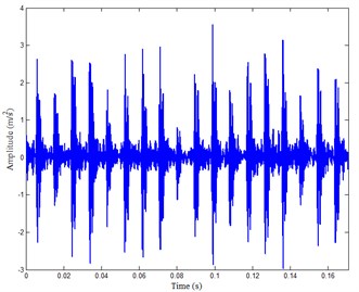
c) Outer raceway faults
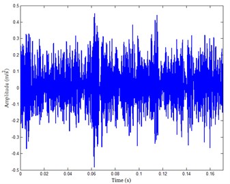
d) Rolling element faults
Fig. 14Comparison of probability density of vibration signals from rolling bearing by two methods
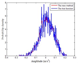
a) Normal running condition
b) Inner raceway faults
c) Outer raceway faults
d) Rolling element faults
Fig. 15Probability density with different divided segments got by the hist function
a) Number of segments is 50
b) Number of segments is 100
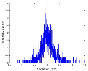
c) Number of segments is 1000
Fig. 16Probability density with different divided segments got by the new method
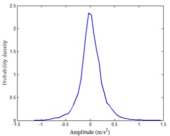
a) Number of segments is 50
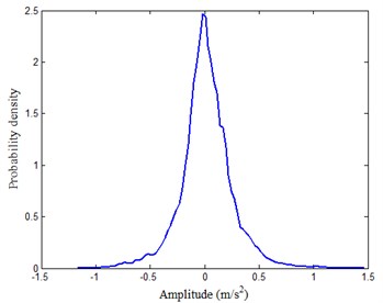
b) Number of segments is 100
c) Number of segments is 1000
8. Conclusions
For the discrete sampling data of a vibration signal, a direct calculation method of probability density based on the LIM is proposed to calculate the probability density. In the new method, the corresponding probability is obtained by using the time got by the LIM, which the amplitude is in some segment ratio to the total observation time of the signal. This method is more accurate than the method using the ratio of sampling points in some segment to the total number of sampling points in MATLAB and LabVIEW. The comparisons among the calculation results of probability density of a sinusoidal signal got by the new method, the methods of MATLAB and LabVIEW show that the direct calculation method based on the time ratio and LIM can both correctly show the probability density curve of a signal, and can solve the problems that the number of sampling points and divided segments would affect the results in the histogram estimation. Another advantage of the new method is that because of no using window function, the results got by the new method will not be affected by the type of window function and window width which are used in the Parzen window density estimation. The calculation results of the probability density of the vibration signals from rolling bearings in different conditions show that the trends of the probability density curves calculated by the new method and that by the hist function are coincident, the influence of the number of segments on the results by the new method is less than that by the hist function. So, the new method based on the LIM is a more accurate method in the probability density calculation than other methods of MATLAB and LabVIEW.
References
-
Li Y. G., Kong X. N., Gao Y. Y. Method for detecting bolt looseness based on probability density of vibration signals of two connected parts and principal component analysis. Journal of Vibration and Shock, Vol. 34, Issue 1, 2015, p. 63-67.
-
Zhang Y. M. Comparative Study of Probability Density Function Estimation Based on Different Kernel Functions. Hebei University, 2015.
-
Li W. Q. Blind Sources Separation Based on Estimation of Probability Density Function of Mixture Signals. Xidian University, 2005.
-
Zhao S. J. Recursive algorithm of detection probability for random phase signals. Journal of Xidian University, Vol. 26, Issue 5, 1999, p. 600-602.
-
Zhi Y. F., Zhang J., Yang B. Z., Zhao N. Novel signal processing method based on maximum likelihood estimator (MLE). Journal of North Western Polytechnical University, Vol. 26, Issue 2, 2008, p. 179-182.
-
Sha Y. D., Guo X. P., Zhao J. Random sonic fatigue life prediction based on stress probability density and power spectral density method. Journal of Vibration and Shock, Vol. 29, Issue 1, 2010, p. 162-165.
-
Xu Y. Z., Bai G. L. Probability density evolution method of fatigue strength-life relationship. Journal of Vibration and Shock, Vol. 32, Issue 8, 2013, p. 35-38.
-
Song L. Y., Chen P., Wang H. Q., Kato Miki Intelligent condition diagnosis method for rotating machinery based on probability density and discriminant analyses. IEEE Signal Processing Letters, Vol. 23, Issue 8, 2016, p. 1111-1115.
-
Song L. Y., Chen P., Wang H. Q. Intelligent diagnosis method using probability density distribution and principal component analysis – application on gear rotating machinery. International Symposium on Flexible Automation, 2016, p. 386-389.
-
Grasso M., Chatterton, Pennacchi, Colosimo B. M. Data-driven method to enhance vibration signal decomposition for rolling bearing fault analysis. Mechanical Systems and Signal Processing, Vol. 81, 2016, p. 126-147.
-
Boškoski Pavle, Juricic Dani Fault detection of mechanical drives under variable operating conditions based on wavelet packet Rényi entropy signatures. Mechanical Systems and Signal Processing, Vol. 31, 2012, p. 369-381.
-
Szolc T., Tauzowski P., Knabel J., Stocki R. Nonlinear and parametric coupled vibrations of rotor-shaft system as fault identification symptom using stochastic methods. Nonlinear Dynamics, Vol. 57, Issue 4, 2009, p. 533-557.
-
Dimentberg M. F. Random vibrations of rotating shaft with non-linear damping. International Journal of Non-Linear Mechanics, Vol. 40, Issue 5, 2005, p. 711-713.
-
Dimentberg M. F. Transverse vibrations of rotating shafts: probability density and first-passage time of whirl radius. International Journal of Non-Linear Mechanics, Vol. 40, Issue 10, 2005, p. 1263-1267.
-
Zhuang Z. M., Li F. L., Wei C. L. Probability density estimation for fault detection. Advanced Materials Research, Vol. 562, Issue 564, 2012, p. 1113-1116.
-
Yang Y. M. Probability theory simulation on MATLAB. China Science and Technology Information, Vol. 22, 2011, p. 61.
-
Zhang X. F., Song H. Problem solution using MATLAB in probability and mathematical statistics. Journal of Qufu Normal University, Vol. 41, Issue 3, 2015, p. 23-27.
-
Wang X. J., Wei Z. K., Huang D. M., Zhang C. K. Probability density testing of engine top combustion pressure by LabVIEW. Agricultural Equipment and Vehicle Engineering, Vol. 3, 2008, p. 13-14.
-
Chu B. Z., Wang C. X. Probability Statistics. Peking University Press, 2010.
-
He Z. J., Chen J., Wang T. Y., Chu F. L. Theory and Application of Mechanical Fault Diagnosis. Higher Education Press, 2010.
-
Ma C. Investigation on Fault Features Extraction for Rolling Bearing and Application. Dalian University of Technology, 2009.
-
Zhang X. G. Pattern Recognition. Tsinghua University Press, 2010.
-
http://csegroups.case.edu/bearingdatacenter/home.
-
Li Y. B., Xu M. Q., Wang R. X., Huang W. H. A fault diagnosis scheme for rolling bearing based on local mean decomposition and improved multiscale fuzzy entropy. Journal of Sound and Vibration, Vol. 360, 2016, p. 277-299.
-
Li Y. B., Xu M. Q., Wei Y., Huang W. H. A new rolling bearing fault diagnosis method based on multiscale permutation entropy and improved support vector machine based binary tree. Measurement, Vol. 77, 2016, p. 80-94.
-
Vakharia V., Gupta V. K., Kankar P. K. A multiscale permutation entropy based approach to select wavelet for fault diagnosis of ball bearings. Journal of Vibration and Control, Vol. 21, 2015, p. 3123-3131.
About this article
The work is supported by the Fundamental Research Funds for the Central Universities (2014MS17).
