Using artificial neural network for forward kinematic problem of under-constrained cable robots

1. Introduction

The first generation of current industrial robots is formed by connecting rigid arms with multiple joints in succession. This conventional structure forms a mechanical arm of open chain series [1]. With the increasing use of robots in various applications, the need for structures that have no limitations of series robots and with special features such as precision, acceleration and high load-carrying capability have been considered more than ever. Parallel robot mechanism is connected end-effector with several closed loop kinematic chain to the base [2]. Due to various weakness of series and parallel robotics such as small workspace, capable of carrying much more than the usual robots and high cost of installation and maintenance, many industries are still not equipped to robotics [3]. To solve this problem, a new class of robots called cable-driven parallel robot were introduced, they are end-loop mechanism which end-effector attached by cable to the base. Each of the cable wrapped around a rotating drum and is connected to the engine by the canvasser cable mechanism, in order to prevent the overlaying of them [4]. Different categories are proposed for cable driven parallel robot based on the number of cables and the number of degrees of freedom of it. The robots are divided to three complete bound robots based on the degree of redundancy including fully constrained robots, over constrained, under constrained. The number of cables is equal to the number of degrees of freedom in the first group, in second group, the number of cables more degrees of freedom and in and third group, the number of cables is less than degrees of freedom [5]. Forward kinematics of parallel robots is to find the position of end-effector using the length of arms which caused to solve dependent nonlinear equations which has no single response in spite of series robots. Given the tension in the cable, in fully constrained robot and over constrained robot, the position of bound full and maximal binding position of the end-only due to the geometry of the robot and the cable specifications can be calculated [6]. While the robot cable tie incomplete due to fixed length cable end-changing forces applied to it varies. The analysis in this article is resolved parallel kinematic robots cable place is unrestricted. Requirements of statics and kinematics equations of incomplete constrained robots can increase the complexity of finding the final position of the robot, when there is a specific set of n variables. It is therefore very difficult to solve the same problem for parallel robots with rigid link. Zhang and Lei [7] presented, the use of neural networks for solving polynomial equations depend on under constrained robots. In this paper, neural network on the information obtained from the inverse kinematics solution was utilized that is much simpler than direct kinematics and is only one answer. Response to neural network has been estimated with a good approximation the forward kinematic robot in a lot of situations, while it should be noted this method, because of the lack of robot equilibrium equations (static) has not required on the accuracy and correctness of it. Yeol et al. [8] proposed a method to solve the forward kinematics of an under constrained cable driven robot. This solution is obtained by finding all balancing situations, similar to rigid four-bar robots. This leads to a non-convex optimization equation, which the minimum value is characterized by changing the initial guess of the optimization process. The limitation of variables caused to change the same optimization problem to a convex optimization problem [9]. The observed value of the optimization problem was considered as a lower limit for the main problem. Meanwhile, author helps the geometry robots to show the mixture of minimum amount of previous work and current minimum. Some similar researches were done in minimization of energy but with this difference that lower bound of optimization problem has obtained by branch and bound algorithm which can compute global minimum of optimization and the height of mass center of end-effector was obtained [10]. Also, this information is useful to make the robot move without hitting the barriers identified above certain constrain. The proposed approach on robots can also be used with a number of more or less cables, which makes it distinct from other solutions. In reference [11], the interval analysis used to find the balance points of end-effectors using a robust and reliable method. As mentioned above, to find the position of the robot, the robot forward kinematic become optimized a question of balance, which aims to minimize the potential energy of end-effector (find the lowest height of the center of mass of the end-effector with the specified cable lengths) and the balance of forces at any moment. This can be conducted using optimization methods such as genetic algorithms or the consideration of changes to variables using convex optimization of analysis and so on. However, the proposed methods are time consuming and are not suitable for practical applications. Li et al. [12] presented a type-2 fuzzy neural network (T2FNN) based inverse control scheme for the level adjustment process. The T2FNN, whose consequent interval weights were trained by the iterative least squares estimation method, was used to approximate the inverse dynamics of the process and to handle uncertainties. Finally, the proposed control scheme and its counterpart type 1 fuzzy neural network based inverse control scheme were compared and implemented for leveling the cable-driven parallel mechanism. Zubizarreta et al. [13] presented the reliable calculation of the direct kinematic problem (DKP) is one of the main challenges for the implementation of real-time (RT) controllers in parallel robots. The DKP estimates the pose of the end-effector of the robot in terms of the sensors placed on the actuators. However, this calculation required the use of time-consuming numerical iterative procedures. In this work, a methodology that used Artificial Neural Networks (ANNs) to approximate the DKP was proposed. Moreover, to demonstrate the effectiveness of the approach, the proposed networks were evaluated considering not only their approximation capabilities, but also their real time performance in comparison with the traditional iterative procedures used in robotics. Boukens et al. [14] presented a robust intelligent controller to be applied to a class of nonholonomic electrically driven mobile robots. the robust adaptive neural network tracking controller developed here introduced adaptive laws to estimate a local upper bound of each subsystem of the nonholonomic mobile robot, then, these laws were used on-line as controller gain parameters in order to robustly improve the transient response of the closed-loop system and reduce conservative, in the sense that the local upper bounds to characterize the corresponding uncertainties dynamics for each subsystem, initially computed based on the worse-case scenario, were not updated during the effective control of the mobile robot. Yang et al. [15] investigated, a novel optimal adaptive radial basis function neural network (RBFNN) control for a class of multiple-input-multiple-output (MIMO) nonlinear robot manipulators with uncertain dynamics in discrete time. To facilitate digital implementations of the robot controller, a robot model in discrete time has been employed. The controller has been designed by an adaptive neural network (NN) based on the feedback system. Son et al. [16] proposed a novel control system combining adaptively feed-forward neural controller and PID controller to control the joint-angle position of the SCARA parallel robot using the pneumatic artificial muscle (PAM) actuator. Reyes and Rosado [17] presented a new polynomial family of PD-type controllers with gravity compensation for the global position of robots manipulators. The previous results on the linear PD controller were extended to the proposed polynomial family. The classical PD controller can be found among this large class of controllers when its proportional gain was a diagonal matrix. Besides the theoretical results, a real-time experimental comparison was also presented to illustrate the performance of the proposed family with other well-known control algorithms such as PD and PID schemes on a three degrees of freedom direct-drive arm. In this paper, in order to solve the cable driven forward kinematics robots, a simulation model was designed in regard to the robot dynamic and behavior of flexible cable with any number of cable driven robot. So, the quasi-static movement of robot in the workspace as well as the effect of gravity and other foreign force on the motion of the robot (the need to minimize the potential energy while quasi-static movement of robot) was designed. The workspace collected forward kinematic data directly from the simulation model and robot position can be obtained at any moment by neural network training with a cable length. The analysis of workspace was conducted in order to show the overall minimum of response. Kumar et al. [18] proposed an online inverse-forward adaptive scheme with a KSOM based hint generator for solving the inverse kinematic problem of a redundant manipulator. In this approach, a feed-forward network such as a radial basis function (RBF) network was used to learn the forward kinematic map of the redundant manipulator. Zhang and Gao [19] developed, a bio-inspired parallel manipulator with one translation along $z$-axis and two rotations along $x$ and $y$ axes as the hybrid head mechanism of a groundhog robotic system. Several important issues including forward kinematic modeling, performance mapping, and multi-objective improvement were investigated with specific methods or technologies. The paper is followed as below, at first the cable driven robot kinematics will be investigated in general and then specifically for cable driven under constrained robots. The simulation model is designed to investigate the end-effector dimensions impact on the expected position of the robot and position has moved for a four cable driven spatial robot. Then to indicate the minimum generality of forward kinematic response, workspace analysis is performed. Finally, in order to ensure this method, the information of trained neural network is used in a control algorithm to control robot position and result is given for a 4 cable driven spatial robot.

2. Cable driven robots kinematics

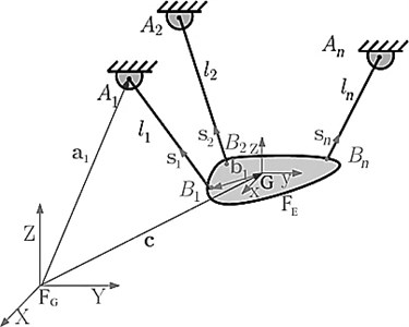
Fig. 1 shows kinematics model of a cable driven robot. ${\mathbf{A}}_i$, ${\mathbf{B}}_i$ ($i=$ 1, 2,…, $n$) are $i$th joint points of cable to base and end-effector. In Fig. 1, ${\mathbf{l}}_i$ is the length vector of $i$ cable and ${\mathbf{s}}_i$ is the unit vector along the ${\mathbf{l}}_i$. $a_i$ and $b_i$ are the connection vectors $A_i$ to the center coordinates vector $G$ (reference) and vector $B_i$ connected to the center coordinates $E$ (attached to the end-effector) respectively. According to Fig. 1, the position of end-effector in $G$ coordinates can be obtained from Eq. (1) [20]:

where, $\mathbf{c}$ is a vector that calculated as two-dimensional position of the robot. Also $R$ is rotation matrix of the coordinate $F_E$ to $F_G$. It is calculted from Eq. (2):

In Eq. (2) $\alpha$, $\beta$ and $\gamma$ are rotation angles around the $x$, $y$ and $z$ axises respectively. with differentiation of Eq. (1), the relationship between velocity of joints and velocity of end-effector is obtained from Eq. (3) [21]:

In Eq. (3), $\dot{\mathbf{L}}={[{\dot{\mathbf{l}}}_1,{\dot{\mathbf{l}}}_2,\dots ,{\dot{\mathbf{l}}}_n]}^T$ is the dispacment vector of the cables length and $\mathbf{t}={\left[\dot{\mathbf{c}\mathbf{}}{\mathbf{\omega }}_i\right]}^T$ is linear vector speed and angular velocity of end-effector. In Eq. (3), $J$ is a jacobian matrix of robot and calculated from Eq. (4) as bellows:

where $s_i$ is unit vector along the $i$th cable.

2.1. Solving the forward kinematics problem of under constrained robots

As mentioned earlier, in order to find the position of under constrained robots, the forward kinematic can be become as an equilibrium problem of optimization, which aims to minimize the energy potential of end-effector (find the lowest height of the center of mass of the end-effector with certain cables length) and the equilibrium of forces at any moment. Eq. (5) shows the mathematical optimization problem of the robot as bellows:

5

$\text{Find:}\mathbf{v}={\left[x,y,z,\alpha ,\beta ,\gamma \right]}^T,\mathit{}\mathit{}\mathit{}\mathit{}{\mathbf{l}}_i=\mathbf{c}+{\mathbf{a}}_i-{{}_{}{}^{F_G}{\mathbf{R}}_{F_E}}^{}\times {\mathbf{b}}_i,$
$i=1,2,\dots ,n,\min \left(ar{g}_z\left(PE\right)\right),\text{s. t.}:{‖{\mathbf{l}}_i‖}^2\le {\mathbf{l}}_i,$
$\mathbf{l}\mathbf{b}\le \left[x,y,z\right]\le \mathbf{u}\mathbf{b},-\frac{\pi }{4}\le \left[\alpha ,\beta ,\gamma \right]\le \frac{\pi }{4},$

where $\mathbf{l}\mathbf{b}$ and $\mathbf{u}\mathbf{b}$ are the lower limit and upper limit of robot position. In addition, PE is the robot's potential energy. Eq. (5) is always in condition of the tension of the cables. To facilitate the understanding of this problem, suppose a body connected to a cable hanging from a fixed point and also with the assumption of tension in this cable which an body can move on a circle equal to the radius of the cable. By releasing of the body will be seen that the tendency of it to the lowest point on the Earth’s gravity (least amount of potential energy).

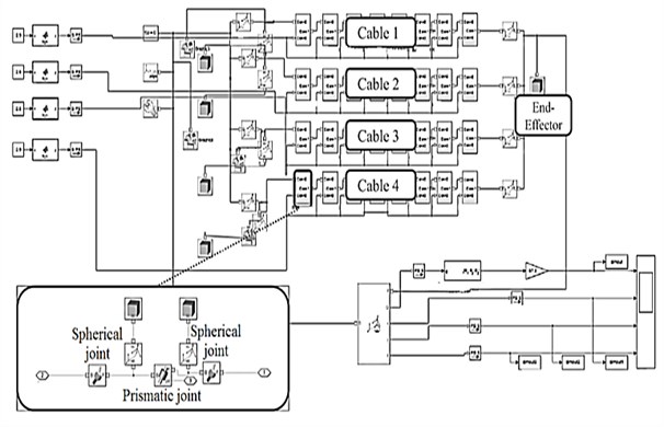
The body will receive to equilibrium at the point of the minimum energy of potential, after a period of oscillation of the body around this point (loss of energy). This problem can be solved by using the optimization methods such as genetic algorithm or the consideration of variable changes of domain using convex optimization, interval analysis and so on. The above methods are time consuming and are not appropriate for practical applications. So, in this paper to solve the forward kinematic of cable driven under constrained robots, a simulation model with respect to the dynamics of the robot and cables is designed to solve the quasi-static motion of the robot in the workspace. The designed simulation model has dynamical and geometric behavior closer to the extendable robot behavior for any cable robot with each number of cable and also with each external force imposed on robot such as gravity force. In addition, in this model by dividing each cable to the elements with mass, the mass and dynamic of the cable have been considered. Fig. 2 shows the model of the robot in SimMechanics environment of MATLAB for a 4 cable spatial robot.

Fig. 1Kinematic model of a cable driven spatial robot with n cables

As shown in Fig. 2, each cable is made of several cylinder joints connected to each other by spherical joints. Due to this, it is necessary by minimizing of the end-effector, so the difference between the expected location and end-effector position due to its mass will be reduced. In Figs. 3 and 4, this problem has been shown for large and small end-effector well. Adding the geometric constraints to the optimization problem of the robot, it will change to a concave optimization problem and can be shown that the answer of this problem is unit and the local minimum is the same to the global minimum in the reachable workspace of the robot with certain cable lengths [10]. In this paper, this theory is shown by using simulation and geometric models. If the end-effector is connected only to one cable, by considering the distance of the mass center of the end-effector to the cable, $b$ and cable length $l$, are an accessible workspace of this system with the assumption of the cable tension, will be in the form of a spherical shell with a maximum radius $l+b$, when end-effector has placed in parallel to the cable, and the minimum radius $\mathbf{l}\mathbf{b}$, when the end-effector placed on the cable. The workspace has been shown in Fig. 5 and mathematical representation is provided in Eq. (6):

6

${\left(x_i-x_{i0}\right)}^2+{\left(y_i-y_{i0}\right)}^2+{\left(z_i-z_{i0}\right)}^2=R_i^2,$
$l_i-b_i\le R_i\le l_i+b_i,i=\mathrm{1,2},\dots ,n.$

Similarly, with the addition number of the cables, the total workspace of the same volume of spheres will be obtained from the intersection of all spheres. It is worth noting, forward kinematics would be answered when all spheres have an intersection. Workspace obtained from spherical shells intersection has a general minimal global point. It simply is visible in Fig. 6.

Also, due to the need to minimize the potential energy of any body, the center of mass of the end-effector intends to get at this minimum point (regarding to the potential energy law, this point is where the mass center of the end-effector has the lowest height). This problem is clear with regarding the results of the simulation in the Fig. 6. As shown in Fig. 7, by releasing the end-effector into the workspace in a simulation environment and adding the loss of the energy terms in the environment, end-effector will move to the point of the lowest potential energy to be fixed at this point. The principle of minimum total potential energy asserts that a structure or a body should displace to a position for minimum total potential energy, which corresponds to a stable configuration of equilibrium. It is a fundamental concept widely used in physics, chemistry and biology.

Fig. 2Mechanical simulation model of the robot in MATLAB software

Through minimizing this criterion, the position and angle of end-effector can be obtained. Leave-one-out-cross validation and external test set validation are carried out to assess the predictive ability of this new criterion. In leave-one-out-cross validation, one sample point is used as the validation data and the remaining sample points are used for regression analysis to obtain the criterion. Then, the self-motion in the joint space [22] is exploited to optimize the total potential energy criterion to predict the position and angle of end-effector at the validation point. This is repeated such that each sample point is used once as the validation data. The average and standard deviation (SD) of the error of the predicted end-effector position and the predicted joint angel are listed in Table 2. It can be seen that the average error of EE position and joint angle are very small. For external test validation, each subject is asked to reach six arbitrary target points except for another sample points. Based on the above observation, multiple linear regression analysis is adopted to obtain the values of undetermined coefficients. The multiple linear regression model is defined as follows:

7

$k={\mathbf{X}}^T\mathbf{B}=b_0+b_{1}x+b_{2}y+b_{3}z,$

where $\mathbf{X}={[x,y,z]}^T$ is the position of the end-effector, and $\mathbf{B}={[b_0,b_1,b_2,b_3]}^T$ are the regression coefficients. The coefficients in Table 1 are used to predict the end-effector at desired path. The desired path of EE is compared with tracked path of EE. The average and standard deviation of the error of the EE position and the joint angel are listed in Table 3.

Table 1The regression coefficients

Subject	$b_0$	$b_1$	$b_2$	$b_3$
$x$	99.85	–0.16	–1.19	1.22
$y$	94.81	–0.80	–1.88	0.44
$z$	130.37	–0.49	–3.07	0.44
$\alpha$	102.83	0.46	–1.67	1.26
$\beta$	132.33	0.01	–2.32	0.60
$\text{γ}$	120.22	0.05	–1.96	1.52

Table 2The average and SD of the error of the end-effector position and the rotation angle in leave-one-out-cross validation

Subject	Position		Joint angle
	Mean (cm)	SD (cm)	Mean (deg)	SD (deg)
$x$	0.43	0.35	1.47	1.17
$y$	0.86	0.80	2.70	4.17
$z$	0.68	0.51	2.10	2.44
$\alpha$	0.66	0.63	2.31	2.02
$\beta$	0.70	0.68	2.23	2.21
$\gamma$	0.62	0.55	3.10	2.73

Table 3The average and SD of the error of the end-effector position and the rotation angle in external test validation

Subject	Position		Joint angle
	Mean (cm)	SD (cm)	Mean (deg)	SD (deg)
$x$	0.44	0.32	1.40	1.08
$y$	0.49	0.58	1.99	2.56
$z$	0.55	0.46	2.19	1.57
$\alpha$	0.72	0.47	2.59	1.71
$\beta$	0.59	0.66	1.77	2.07
$\gamma$	0.53	0.42	1.03	2.08

It can be seen that the average error of EE position is less than 1 cm while the average error of EE position predicted by the criterion of minimization of the norm of joint angular velocities is larger than 4 cm. All these results prove the validity of the total potential energy criterion.

2.2. LOLIMOT algorithm

In this paper, using a pre-trained neural network, the position and angles of end-effectors are calculated with acceptable error. One of the most commonly useful algorithms for changing complex models to smaller and linear models is known as LOLIMOT. LOLIMOT (Local Linear Model Tree) is an incremental tree construction algorithm which partitions the input space by axis-orthogonal split. This technique is also known as locally linear neuro-fuzzy (LLNF) identification method. In each iteration, a new rule or local linear model is added to the model and the validity function which is corresponded to the actual partitioning of the input space are computed and the corresponding rules are optimized using a local weighted least squares technique. Therefore, the algorithm avoids time consuming nonlinear optimization [23]. The main idea of LLNF is the approximation of a nonlinear function with dividing the input space to the small linear subspaces using fuzzy fitness. Therefore, each of these subspaces can be described with a fuzzy neuron and each fuzzy fitness function creates a locally linear model. The fuzzy fitness function is assumed to be Gaussian fuzzy function which is given below:

8

$\mu \left(x\right)=\exp \left(-\frac{{\left(x-c\right)}^2}{{2\sigma }^2}\right).$

LOLIMOT algorithm has two loops: outer loop and inner loop. Nonlinear parameters or primary rules, which are known as model structure, are computed in outer loop and secondary parameters which are linear parameters, are determined in inner loop. LLNF output is determined by weighted summation of all neuron outputs, as follows:

9

${\widehat{y}}_i={\omega }_{i0}+{\omega }_{i1}{u}_1+\dots +{\omega }_{ip}{u}_p,$

10

$\widehat{y}=\sum _{i=1}^M{\widehat{y}}_i{\mathrm{\varnothing }}_i\left(\underset{\_}{u}\right).$

The model structure of this algorithm is shown in Fig. 8. The algorithm starts with optimum least square estimation, and for decreasing prediction error creates a locally linear neuron. A neuron which has the worst estimation error, is the candidate for division at the end of each iteration. The portion for division of each nominated neuron is 1/2; it means selected neuron is divided into two equal neurons. New center and standard deviation for these fitness functions is updated. As it mentioned previously, normalized orthogonal Gaussian functions are used as fitness functions. In this case, normalization is a necessary requirement for fitness function definition which is described, as follows:

11

${\mathrm{\varnothing }}_i\left(\underset{\_}{u}\right)=\frac{{\mu }_i\left(\underset{\_}{u}\right)}{\sum _{j=1}^M{\mu }_j\left(\underset{\_}{u}\right)},$

12

${\mu }_i\left(\underset{\_}{u}\right)=\exp \left(-\frac{1}{2}\left(\frac{{\left(u_1-c_{i1}\right)}^2}{{\sigma }_{i1}^2}+\dots +\frac{{\left(u_p-c_{ip}\right)}^2}{{\sigma }_{ip}^2}\right)\right).$

According to Eq. (12), each weighted Gaussian function has two sets of nonlinear parameters; $c_{ij}$’s are centers and ${\sigma }_{ij}$’s are standard deviations for each $M$ neurons. Nonlinear parameters of fitness function are determined using learning or optimization methods, and secondary parameter for each LLNF is estimated via local weighted least squares technique separately [23]. These weights are elements of the following matrix with $M\times (p+1)$ dimension:

13

$\underset{\_}{\omega }=[\begin{array}{ccc}{\omega }_{10}& {\omega }_{11}& \begin{array}{cc}\cdots & \begin{array}{ccc}{\omega }_{1p}& \begin{array}{cc}{\omega }_{20}& {\omega }_{21}\end{array}& \begin{array}{cc}\cdots & \begin{array}{cc}{\omega }_{M0}& \begin{array}{cc}\cdots & {\omega }_{Mp}]\end{array}\end{array}\end{array}\end{array}\end{array}\end{array}.$

And, regressors for $N$ samples are as follows:

14

$\underset{\_}{X}=[\begin{array}{ccc}{\underset{\_}{X}}_1& {\underset{\_}{X}}_2& \begin{array}{cc}\cdots & {\underset{\_}{X}}_M\end{array}]\end{array},$

where:

15

${\underset{\_}{X}}_i=\left[\begin{array}{ccc}\begin{array}{c}{\mathrm{\varnothing }}_i\left(\underset{\_}{u}\right(1\left)\right)\\ {\mathrm{\varnothing }}_i\left(\underset{\_}{u}\right(2\left)\right)\end{array}& \begin{array}{c}{u_1\left(1\right)\mathrm{\varnothing }}_i\left(\underset{\_}{u}\right(1\left)\right)\\ {u_1\left(2\right)\mathrm{\varnothing }}_i\left(\underset{\_}{u}\right(2\left)\right)\end{array}& \begin{array}{cc}\cdots & \begin{array}{c}{u_p\left(1\right)\mathrm{\varnothing }}_i\left(\underset{\_}{u}\right(1\left)\right)\\ {u_p\left(2\right)\mathrm{\varnothing }}_i\left(\underset{\_}{u}\right(2\left)\right)\end{array}\end{array}\\ ⋮& ⋮& ⋮\\ {\mathrm{\varnothing }}_i\left(\underset{\_}{u}\right(N\left)\right)& {u_1\left(N\right)\mathrm{\varnothing }}_i\left(\underset{\_}{u}\right(N\left)\right)& \begin{array}{cc}\cdots & {u_p\left(N\right)\mathrm{\varnothing }}_i\left(\underset{\_}{u}\right(N\left)\right)\end{array}\end{array}\right],$

16

$\widehat{\underset{\_}{y}}=\underset{\_}{X}\widehat{\underset{\_}{\omega }},\widehat{\underset{\_}{\omega }}={(\underset{\_}{X}}^T{\underset{\_}{X})}^{-1}{\underset{\_}{X}}^T\underset{\_}{y}.$

Finally, the LOLIMOT algorithm according to [23] can be summarized as follows:

1) Initial model: in the started model, $M=$ 1 and ${\mathrm{\varnothing }}_1\left(\underset{\_}{u}\right)=$ 1; a locally linear neuron is globally estimated for the whole input space. Then iterate as follows:

2) Finding the worst neuron: The neuron which has minimum efficiency is found by evaluating Mean Square Error (MSE) for all $M$ neurons.

3) Checking all possible direction: selected neuron fitness function should be tested by dividing into two parts in all possible P directions as these steps:

3.1) Create fitness functions for every two new neurons.

3.2) Estimate secondary parameters locally for every two new neurons.

3.3) Compute the total cost function for the model.

The third step in the proposed modeling algorithm is LOLIMOT training. Different numbers of neurons are checked to get the best results to minimize a performance index. The performance index can be selected among ME, MSE or SCC which are introduced in the following:

Max Error (ME): This index is defined, as follows:

17

$ME=Max\left|P_{Tracked,i}-P_{Desired,i}\right|,i=\mathrm{1,2},\dots ,N,$

where, $P_{Tracked,i}$ is the actual value of robot output path for the ith point in testing dataset and $P_{Desired,i}$ is the output of LOLIMOT model and $N$ is the number of dataset samples.

Mean Square Error (MSE): This index is used to study the quantity differences between outputs of LOLIMOT models and actual values of robot outputs. Therefore, this index can measure the average of the squared error which is defined, as follows:

18

$MSE=\frac{1}{N}\sum _{i=1}^N{(P_{Tracked,i}-P_{Desired,i})}^2.$

The better predictive ability of the model in prediction makes both indices closer to 0.

Squared Correlation Coefficient (SCC): This index is used for defining variability in a dataset. SCC can be used for demonstrating the correlation between predictive values and actual values. On the other hand, SCC shows how good a predictor might be constructed from the output model values [24, 25]. This index can be varied from 0 to 1. Better predictive ability of LOLIMOT-based model makes this index nearer to 1.

4) Finding the best deviation: the direction that produces the minimum error is selected. After increasing the division number of neurons from $M$ to $M+1$, the algorithm is come back to the second step until the learning algorithm is stopped.

Stopping condition can be reached for a predetermined error between output ($y$) and LLNF output $\left(\widehat{y}\right)$, it means when:

$‖y-\widehat{y}‖<\epsilon .$

In this paper, a four cable spatial robot with physical geometry specification is shown in Fig. 9 and the simulation model was developed. In Table 4, vectors $\mathbf{a}$ are in the global coordinate. Also, vectors $\mathbf{b}$ are in moving coordinate attached to the end-effectors. About 35000 reachable workspace of the robot (this workspace is obtained from the limiting angles of robot less than 45 degrees) were collected. In this method, at first it is supposed the correctness of cable robot inverse kinematics, then the workspace was covered using layer to layer and linear movements.

Table 4Physical and geometrical specifications of cable driven robots

Value	Parameter / vector
[–130, 220, 240]	$a_1$(m×10-3)
[110, –260, 235]	$a_2$ (m×10-3)
[130, –310, 210]	$a_3$ (m×10-3)
[–130, –315, 200]	$a_4$ (m×10-3)
[–20, 20, 0]	$b_1$ (m×10-3)
[15, 20, 0]	$b_2$ (m×10-3)
[15, –20, 0]	$b_3$ (m×10-3)
[–20, –20, 0]	$b_4$ (m×10-3)
800	$m$ (kg×10-3)
11	$I_{xx}$ (kg·m2×10-3)
11	$I_{yy}$ (kg·m2×10-3)
8	$I_{zz}$ (kg·m2×10-3)

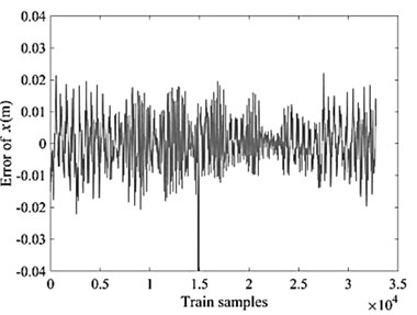
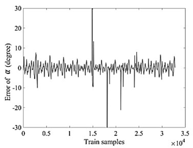
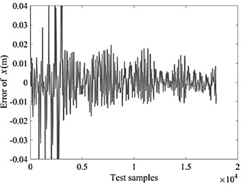
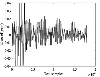
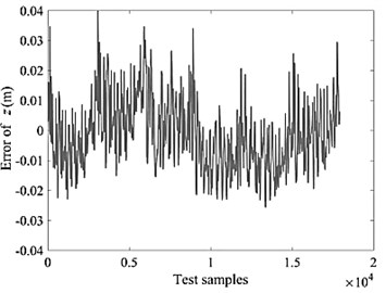
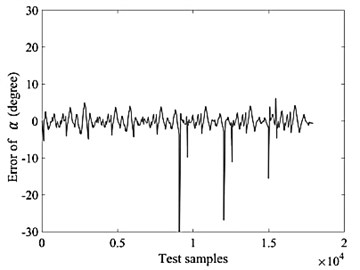
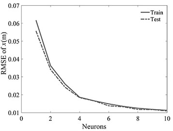
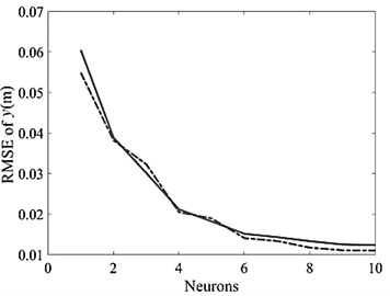
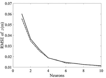
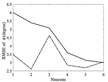
So, the length of the cables was determined by this method as the input of virtual robot model and angles as well as positions were collected. Due to the length of cables as neural network input and six degrees of freedom, including positions and angles as output, the network was trained. Less than 20000 of 35000 collected data were selected for train samples and about 8000 dates to test samples. It is worth noting that in LOLIMOT neural network to train samples, the network is trained once for each output. In the Figs. 10 and 11, the tracking error for each output parameters are given for training and testing data. Also in Figs. 10 and 11, the number of neurons devoted to train for each of the outputs, and root mean square error are provided. As shown in the Figs. 10 and 11, the position error is about 2 cm and the angles error is about 5 degrees, which is acceptable due to the big area of the workspace [26, 27].

Fig. 5The workspace of each taut cable

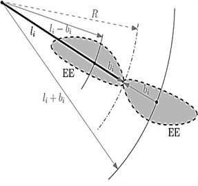
Fig. 6Robot workspace for specified cable length

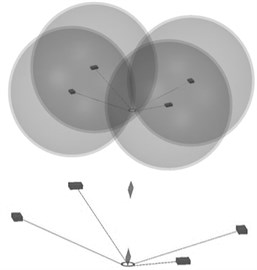
Fig. 7The end-effector movement toward the minimum potential energy

a)

b)

c)

d)

A grid search is performed to select the best number of neurons for dynamic modeling of robot. It is observed that the best number of neurons is 10. Fig. 12 shows that using this number of neurons causes less error in prediction of output path and rotation of the robot. For the proposed LOLIMOT-based model, ME, MSE and SCC are 1.46, 0.4310, and 0.9988, respectively. It can be seen that the trained LOLIMOT has acceptable results in this area.

Fig. 9Structure of spatial robot with a four cable

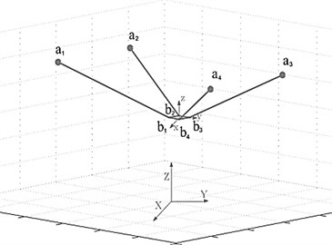
Fig. 8Model structure of LOLIMOT algorithm

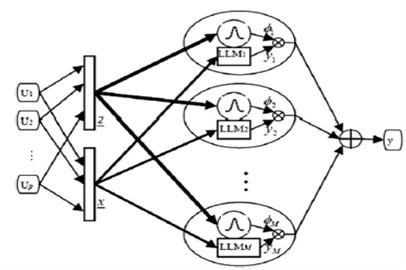
Fig. 10NN training data error

a)

b)

c)

d)

3. Robot control

Fig. 13 shows the control algorithm of this paper. In this algorithm, the optimal inputs are $x$, $y$ and $z$ because only four degrees of freedom due to the 4 operator can be controlled, so only robot positions are important for us. Since feedback to robot position of forward kinematics can be compensated by space error, we can assume the end-effector as a concentrated point with weight. As a result, inverse kinematics equations will be attached only the robot position (not angle). With this assumption in Eq. (1), $b$ will be zero, also Jacobin robot will become 3×$n$ matrix instead of a 6×$n$ matrix and Jacobin matrix is calculated from Eq. (19) as bellows:

The proposed controller not only keeps all cables under tension for the whole workspace of the robot, it is chattering-free, computationally simple and it does not require measurement of the end-effector acceleration. The effectiveness of a control strategy in a pre-grasping operation can be positively evaluated when some requirements on the kinematic and dynamic state of the end-effector and the target are satisfied (the adopted threshold values are reported within parentheses):

1. During the maneuver the distances between the end-effectors and the target are null or within a prescribed tolerance (of the order of centimeters);

2. During the maneuver the end-effector shows relatively small translational position magnitude and angular displacements (respectively 2.1 cm and 1.2 deg);

3. Conditions 1 and 2 are maintained for a prescribed time interval (of the order of 20 sec.)

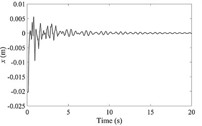
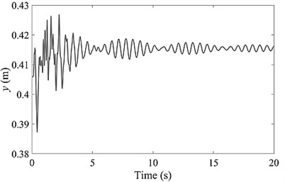
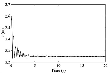
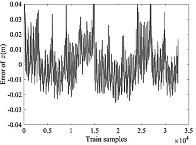
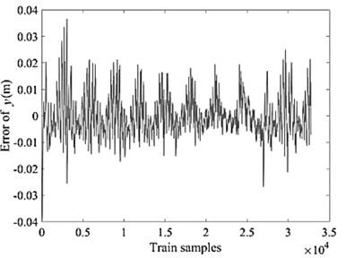
The final position of the robot obtained using neural network and this value is compared with closed-loop of the desired value. Trying to eliminate the error obtained of PD controller with coefficients $k_p=$ 2.34 and $k_d=$ 0.17 is done. Proportional-Derivative or PD control combines proportional control and derivative control in parallel. Proportional-derivative control is useful for fast response controllers that do not need a steady-state error of 0. It is a controller can be used to make a simple system track some reference point. The mentioned control algorithm has been done in MATLAB software. As shown in Figs. 14, 15 and 16, tracking error for helical path is about 2 cm in the worst case which is acceptable due to the big workplace of robots. In Fig. 17, the desired path and the tracked path of the robot is given in a 3D graph. Fig. 17 shows a good performance of controller.

Fig. 11NN testing data error

a)

b)

c)

d)

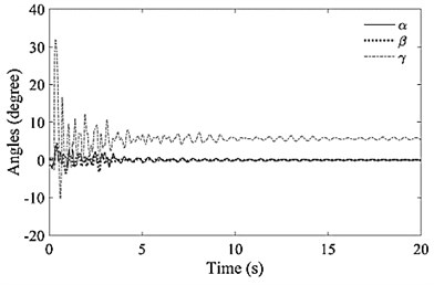
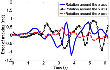
In this research, we have used from Integral Square Error (ISE), Integral Time Square Error (ITSE) and Integral Absolute Error (IAE) for comparing the error of controller. From IAE criterion, the error value is the same from the beginning to the end of the path, and this criterion measures the difference between the absolute value of the desired path and tracked path. From ISE criterion, the significance of the error from the beginning to the end of the path is not the same. The less error is, the less important its importance, and this difference in significance is such that small errors are almost incrementally increasing with the second-power error ratio. From ITSE, the significance of the error at the beginning and the end of the path is not the same. In this criterion will increase the importance of the error by increasing the time it takes, and the final error rate of the system will be significant. Table 5 shows the error valve of this controller for the robot. In addition, Fig. 18 shows the error of tracking desired trajectory rotation around the $x$, $y$ and $z$ axes with PD controller.

Fig. 12Optimal number of neurons for LOLIMOT

a)

b)

c)

d)

Fig. 13Suggested control block diagram for control of robot position

Fig. 14Tracking error of a helical path in x direction

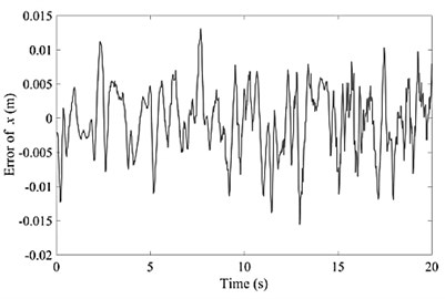
Fig. 15Tracking error of a helical path in y direction

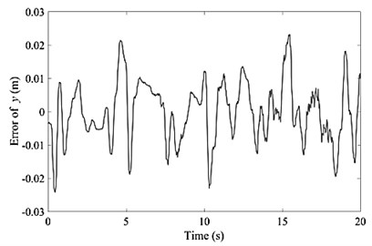
Fig. 16Tracking error of a helical path in z direction

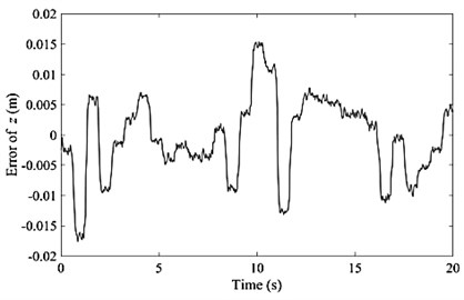
Fig. 17Comparison of end-effector path with optimal path

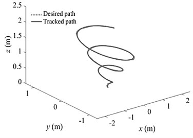
Fig. 18Error of tracking desired trajectory rotation around the x, y and z axes with PD controller

4. Conclusions

In order to find the end-effector position of under constrained robots at any moment and the use of it in the control algorithms, a method based on neural network algorithms was proposed. This paper has introduced a new algorithm for position control of end-effector, it is a PD-type controller. It is supported by a rigorous stability analysis, the theoretical results establish conditions for ensuring global regulation. The simple PD controller can be a particular member of this new scheme when its proportional gain is a diagonal matrix. For stability purposes, the tuning procedure for the new scheme is sufficient to select a proportional gain as diagonal matrix and derivative gain as symmetric positive definite matrix in order to ensure global asymptotic stability. At the same time due to the necessity of taking into account the geometry and static of under constrained robots, forward kinematics became an optimization problem for minimizing the potential energy of the robot. Given the time-consuming and dependent on the initial value of solving the optimization problem, this method is not suitable for practical applications. In order to solve this problem, using the neural network, a simulation of learning process is carried out based on the environmental data and the results were used in the control algorithm simultaneously. Network error in the workspace of the robot was obtained 0.38 percent in positions and approximately 3.87 % for angles, respectively. The simulation model is very exact and can consider robots and cable dynamic for each cable driven robots in each number of cables. Note that the new algorithm improves the performance obtained by PD and neural network controllers. The family of proposed controllers effectively exploits its exponential capability in order to enhance the position error, having a short transient phase and a small steady-state error. Fast convergence can be obtained (faster response). Consequently, the control performance is increased in comparison with the aforementioned controllers. In addition to considering the impact of external forces acting on the robot, it is not necessary to use various expensive sensors to obtain the position of the robot. To show the unique and global minimum of achievement response, the analytic workspace was done. Using data from the trained neural network, the control algorithms are designed and implemented in MATLAB simulation environment. Due to the large working space of the robot, the error is very good and acceptable. The results show that the good performance of this method.