Research and application of Volterra series theory in rolling bearing fault state feature extraction

1. Introduction

Rolling-element bearings, also called rolling bearings, are the core components of rotating machinery. When failure of a rolling bearing occurs, the vibrational signal is usually strongly non-linear with non-stationary features [1, 2].

Therefore, it is possible to extract the fault characteristics from this type of signal in order to accurately differentiate fault types and failure development trends. Traditional feature extraction methods for nonlinear non-stationary signals have included the wavelet transform (WT) [3-5], singular value decomposition (SVD) [6], empirical mode decomposition (EMD) [7, 8], and the Hilbert-Huang transform [9]. While these methods have been widely used, they do not provide complete extraction of the fault information and exhibit or adaptive filtering. Moreover, nonconformity of the fault frequency drift can occur due to the existence of bias in the simplified mechanical model established using the theoretical failure values and actual system outputs.

A number of time-frequency manifold (TFM) techniques have been proposed [10] including the use of cross features from nonlinear data [11], chaotic feature space [12], ICD and adjustable Q-factor wavelet transforms [13], dominant trend based logistic regression (DTLR), transient modeling, and the new non-linear time-frequency feature extraction method using the Levenberg-Marquardt (LM) method for parameter identification [14]. However, most of the above methods have only been optimized for feature extraction from the vibrational data obtained under certain conditions and using specialized equipment. Optimization of a number of factors have not previously been considered: 1) theoretical mechanics to simplify the model and real system error; 2) the fault characteristic signal of the nonlinear non-stationary case; and 3) the fault trend evolution.

Based on the fault feature extraction method of the Volterra series kernel model and the multi-pulse excitation method, a different method of fault information feature extraction is proposed using a nonlinear transfer function [15, 16]. The output signal can be used to establish a non-linear closed-loop system [17] to accurately describe the transmission characteristics of a nonlinear bearing system. In the fault diagnosis model [18-21], the Volterra time domain kernel (GIRF) and frequency domain kernel (GFRF) can be used to determine the dynamic characteristics of a nonlinear system. The problem of intuitionistic representation of the time and frequency domain kernel function was solved using the bispectrum method [22-24] and the validity of the method was verified experimentally.

2. The multiple excitation algorithm

The Volterra series can be theoretically determined using numerical algebra and infinite length algebraic sum of the multidimensional convolution. The specific formula is defined as:

where $h_k({\tau }_1,{\tau }_2,...,{\tau }_k)$ is the core of the $k$-th order Volterra series.

From the above equation, the kernel is the key to solving the series development, and thus the foundation of the series element. For a discrete nonlinear time invariant system, the series can be represented as:

In order to ensure operability, system modeling should be carried out within certain value limits. The effects are not calculated based on the dc component such that Eq. (2) can be rewritten as:

where $N$ is the highest order of the non-linear system, $M$ is the length of memory of the impulse response, and $e\left(k\right)$ is the truncation error. Assuming the system is nonlinear, Eq. (3) can be used and the first unit of a certain gain pulse will be the system input, namely, ${\mu }_0\left(t\right)=a_{\delta }\delta \left(t\right)$ the following formulae can then be used to determine the first-order kernel of the system:

where $a_{\delta }$ is the pulse stimulated amplitude.

From the equation:

There are both $h_1\left({\tau }_1\right)$ and $h_2({\tau }_1,{\tau }_2)$ assuming of the Volterra series of the kernel, with two different incentives as input to solve and discuss. The final formula is given as follows:

Expressed in matrix form and substituting Eqs. (7)-(10) into the following formula:

where $h_1\left(\tau \right)$ can be written as:

In the same way, $h_2({\tau }_1,{\tau }_2)$ can be represented by:

Given $h_1\left({\tau }_1\right)$, $h_2({\tau }_1,{\tau }_2)$ and $h_3({\tau }_1,{\tau }_2,{\tau }_3)$ and assuming the Volterra series kernel, the series can be written as:

where $h_3({\tau }_1,{\tau }_2,{\tau }_3)$ is the third order time domain kernel of the non-linear system.

Using three different pulse excitations $h_1\left({\tau }_1\right)$, $h_2({\tau }_1,{\tau }_2)$, and $h_3({\tau }_1,{\tau }_2,{\tau }_3)$ as the input signals, the series can be solved using the following formula:

Based on the Vandermonde matrix and using the numerical method to solve the Volterra first-order kernel, the formula can be represented as:

In the same way, we get:

Different pulse excitation inputs into the system will result in different Volterra series outputs. If the system input is greater than the third-order pulse, i.e., an advanced kernel, then the model becomes computationally intensive and solving the inverse matrix $\left[AB\right]$ of the coefficient matrix ${\left[AB\right]}^{-1}$ falls into the curse of dimensionality.

3. Verification of the method

For any continuous nonlinear time invariant system under initial conditions equal to zero, the input signal energy is limited to the system response that can be described by the Volterra series. It is assumed that there exists a linear single degree of freedom function, as shown by:

where $f\left(y\right)$ is always present and unique within the domain of definition.

When time $t=T$, the pulse excitation is the input function of the system $u\left(t\right)$ and the input function can be described by the following:

where $a_{\delta }$ is the pulsed excitation amplitude.

When the system reaches $t=T$ at amplitude $a_{\delta }$ after the stimulation, the system will produce a finite amplitude jump in response to:

where $y\left(T^{+}\right)$ represents the system response after excitation $T$ and $y\left(T^{-}\right)$ is the system response before excitation $T$.

Integrating from $t=T^{-}$ to $t=T^{+}$, it is possible to simulate the response of the system at the approximate time $t=T$. Eq. (21) can then be converted to:

where $\mu \left(t\right)=a_{\delta }\delta (t-T)$ will produce a discontinuous system response, given by:

According to the above equation, the input function can be expressed as a piecewise function according to the time of the pulse excitation function applied to the system:

Eq. (24) can be approximated to simulate the system impulse input excitation function $\mu \left(t\right)=a_{\delta }\delta (t-T)$ at $t=t_{\delta }$ and width $2{\omega }_{\delta }$. Integrating Eq. (24), it can be found that the maximum value of the impulse excitation $\mu \left(t\right)$ appears at $t=t_{\delta }$, and the derivative at the boundary is zero at $t_{\delta }\pm {\omega }_{\delta }$.

Based on the above analysis, when the system exhibits a pulse function, the response status approaches the ideal unit pulse. By applying multiple pulse excitation to the system, the theoretical change in response of the system state is also close to the ideal unit impulse. Therefore, a solution based on the pulse input using the theoretical kernel method from theory to data calculation is feasible and $\mu \left(t\right)=a_{\delta }\delta (t-T)$.

4. Wavelet comparison experiment

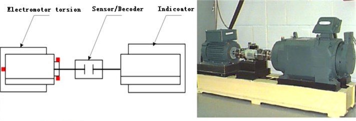
To experimentally validate the model, a test bench (Case Western Reserve University) was used, as shown in Fig. 1. The setup included a 2 HP motor (1.5 kW), torque sensor/decoder, power meter, and electronic controller (not shown in the figure). The bearing support was attached to the shaft of the motor, drive-end bearing for SKF6205, and fan end bearing for SKF6203, and the ball bearing damage point was detected at three different positions: 90°, 0°, and –90°. An acceleration sensor was placed above the fan end of the motor and drive end bearing and used to collect the fault vibration signal of the bearing. The vibration signal was recorded using a 16-channel recorder, and power and speed were both measured using a torque sensor. A normal bearing and ball bearing were chosen for the analysis, and data was obtained using a load of 1492 W and a speed of 1750 r/min.

Fig. 1Rolling bearing fault simulation test bench

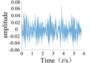
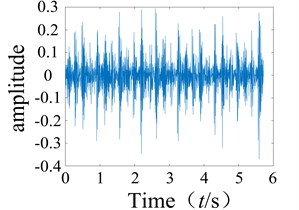
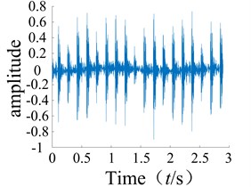
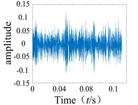
A wavelet transform was adopted to diagnose the ball bearing signal. The wavelet base was used for the signal decomposition and to amplify the signal of the failure of the bearing in order to determine the failure frequency. Since the working frequency and bearing failure frequency are small, the low frequency range signal was amplified. The signal was then decomposed into four layers by the wavelet transform, and analyzed using Hilbert envelope spectral analysis.

Fig. 2Fault bearing wavelet decomposition and feature spectrum diagram

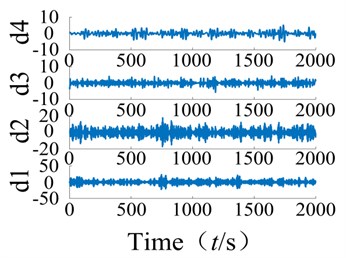
a) 4 layer wavelet decomposition

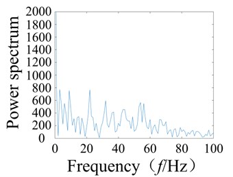
b) Spectrum

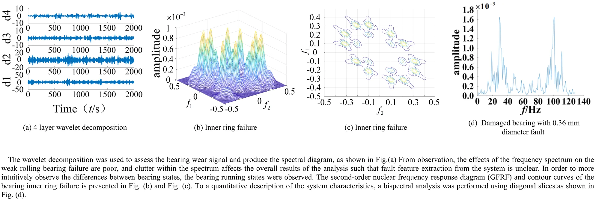
The wavelet decomposition was used to assess the bearing wear signal and produce the spectral diagram, as shown in Fig. 2. From observation, the effects of the frequency spectrum on the weak rolling bearing failure are poor, and clutter within the spectrum affects the overall results of the analysis such that fault feature extraction from the system is unclear. Moreover, when using the system signal based on the wavelet analysis, the corresponding wavelet base must be selected based on practical experience. This is significant since the selected wavelet base will strongly affect the system. Therefore, to obtain accurate results from the analysis, the correct wavelet base must be chosen, and this process of fault diagnosis can be tedious.

5. Experimental demonstration of the proposed Volterra series method

The Volterra series kernel can be assessed using the multi-pulse excitation method to avoid the disadvantages associated with the wavelet decomposition. Using the signal collected from Case Western Reserve University and based on the multi-pulse excitation method, the Volterra series kernel was used to investigate a normal bearing and ball bearing. Three conditions were used: a memory length of the first-order time-domain kernel of 8 and length of the kernel vector of 8; memory length of the second-order time-domain kernel of 5 and kernel vector length of 15; memory length of the second-order time-domain kernel of 5 and vector length of 35.

The multi-pulse excitation method was used to analyze the rolling bearing signals, and it was assumed the series kernels $h_1$, $h_2$, and $h_3$ were present. First, the system inputs a pulse excitation function ${\mu }_0\left(t\right)=\delta \left(t\right)\text{,}$ and the system output is $y_0$. Then, the two pulse excitations are applied to the system $u_1\left(t\right)=\delta \left(t\right)+\delta (t-T)\text{,}$ where $T$ represents the pulse time delay, and the system generates another output $y_1\left(t\right)\text{.}$ Similarly, three additional pulses $u_2\left(t\right)=\delta \left(t\right)+\delta (t-T)+\delta (t-2T)$ with delayed impulses were applied to the system and again, the system generated the output $y_2\left(t\right)$.

The second-order time-domain kernel of the system can be obtained using Eq. (17). The multi-pulse excitation method was used to analyze the rolling bearing signals from the experiment, and a Matlab simulation was then used to obtain the second-order time-domain kernel characteristic curve as shown in Fig. 3. It can be observed that the second-order nuclear time domain spectra of the normal bearing and faulty bearing are clearly different as the numbers of sharp points on each spectrum are quite distinct.

Fig. 3Normal bearing and different periods during failure of the second order nuclear time-domain response

a) Normal bearing

b) Inner ring failure

c) Outer ring failure

d) Roller failure

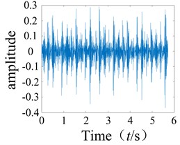
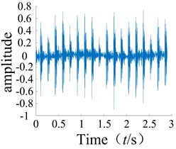
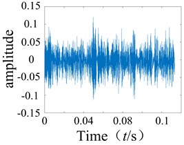
A comparison of the normal bearing and faulty bearing using the second-order time domain is presented in Fig. 4. It was found that the frequencies at which the highest peak appear are 0.3 Hz, 0.8 Hz, and 0.1 Hz. The sites of failure can be clearly distinguished, and directly show huge differences in frequency between the highest peaks and different fault areas on the bearing.

Fig. 4Response of second order nuclear time domain in different parts

a) Inner ring failure

b) Outer ring failure

d) Roller failure

After several tests, it was found that the first-order time-domain kernels of the normal condition and the faulty condition were very similar for the time domain kernel (GIRF), and therefore difficult to distinguish. As such, they will not be discussed further in this paper. The graphs of the second-order kernel clearly show differences in the spikes on the graphs of the faulty bearing compared to the normal bearing (Figs. 3-4), and the number of spikes is greater for the faulty bearing. It was shown that non-linear faults could be detected using the low order kernel of the Volterra series.

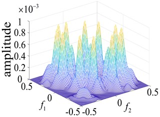
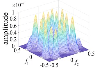
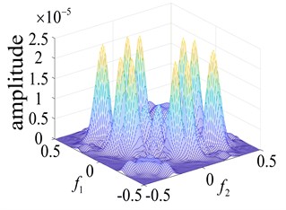
Fig. 5Curves of the normal bearing and different parts of the faulty bearing based on the second order nuclear frequency domain response

a) Normal bearing

b) Inner ring failure

c) Outer ring failure

d) Roller failure

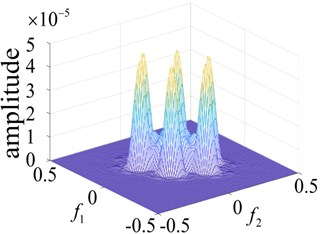
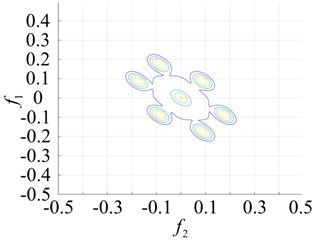
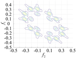
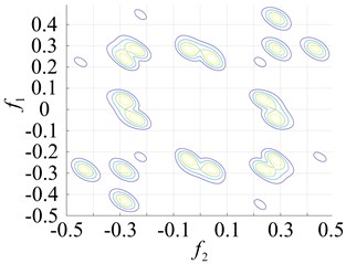
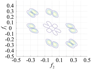
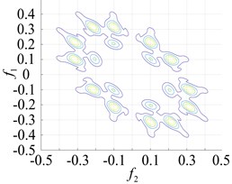
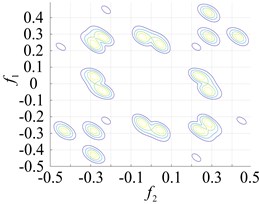
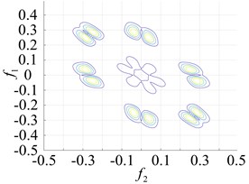
In order to more intuitively observe the differences between bearing states, the bearing running states were observed. The second-order nuclear frequency response diagram (GFRF) and contour curves of the normal bearing and bearing inner ring failure, outer ring failure and ball bearing failure, are presented in Figs. 5-6. It can be observed that the second-order nuclear frequency domains of the normal and faulty bearings are clearly different. The bearing failure site is more clearly seen in the response contour curves. The frequency domain response diagram and second-order core contour figure effectively shows the position of the frequency secondary coupling, and can therefore confirm that the characteristics of the normal bearing and different parts of the faulty bearing system are fundamentally different.

Fig. 6Contours of the normal bearing and different parts of the faulty bearing based on the second-order amplitude-frequency domain response

a) Normal bearing

b) Inner ring failure

c) Outer ring failure

d) Roller failure

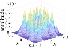
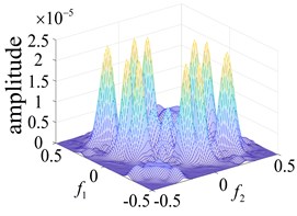
A comparison of the normal bearing versus different parts of the faulty bearing, based on the second-order frequency domain, are shown in Fig. 5. It was found that the frequency points at which the highest peaks appear are at 3.5×10⁵ Hz, 0.8×10³ Hz, 0.8×10² Hz and 2.0×10⁵ Hz. This is consistent with theoretical calculations of the frequency of failure according to frequency and peak number, and can clearly distinguish between the normal and faulty bearings (Fig. 6). The second-order amplitude-frequency response profile of the normal bearing and different parts of the faulty bearing clearly show differences in the number of peaks and the dispersions of the spectra vary greatly. The second-order nuclear frequency domain diagram of the faulty bearing and its separate components depict the differences in system characteristics between the bearings.

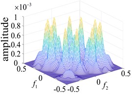
Fig. 7Response of the second order nuclear frequency domain in different parts of the rolling bearing

a) Inner ring failure

b) Outer ring failure

c) Roller failure

The points at which the highest frequency peaks appear were found at 0.8×10³ Hz, 0.8×10² Hz and 2.0×10⁵ Hz (Fig. 7(a) and Fig. 5(b) and (c)). An intuitive description of the different parts of the fault bearing showing the peak frequency points suggest the difference is very clear. The degree of each coupling difference is presented in Fig. 8, which clearly shows the sites of failure.

Based on the Volterra series rolling bearing fault diagnosis, the multi-pulse excitation method can adequately represent the nonlinearity of the system. For different types of system, the method can be used to determine changes in the system using the second order Volterra time domain kernel and third order Volterra time domain kernel. Alternatively, the frequency domain kernel can be used under circumstances where the first order Volterra time domain kernel is difficult to determine, thereby providing richer fault information. It can also be used to determine the operating state of the system via changes in the Volterra nuclear frequency domain figure, obtained using the unique pulse excitation method (Fig. 7).

Fig. 8Contours of the different faulty bearing parts for the second-order amplitude-frequency response

a) Inner ring failure

b) Outer ring failure

c) Roller failure

6. Fault quantification and anti-noise analysis

6.1. Quantitative study on the fault evolution

In this paper, the normal bearing and bearings with roller faults of various sizes, fault diameters of either 0.18 mm or 0.36 mm and a fault depth of 0.28 mm, were used. The drive load was taken as 0 and the drive speed set to 1797 r/min. The input signal to the system was either set to $\sigma \left(t\right)$ or $\sigma \left(t\right)+\sigma (t-1)$, and as the system was run, the vibration output signal was collected using an acceleration sensor. Experimental data were sampled, and 2000 sets of data were intercepted in the sample data for simulation analysis. The multi-pulse excitation method was then used to analyze the input and output data in MATLAB, and the characteristics of the normal bearing and roller fault bearing systems were determined, based on the Volterra kernel functions of $h_1$ and $h_2$, and using the second-order nuclear of $h_2$.

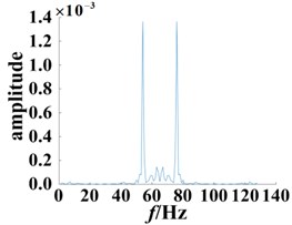
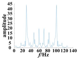
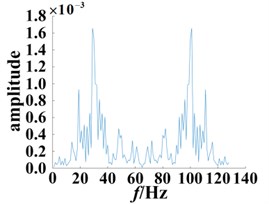
Fig. 9Slices of bispectrum based on the second-order kernel

a) Normal bearing

b) Damaged bearing with 0.18 mm diameter fault

c) Damaged bearing with 0.36 mm diameter fault

The bispectrum three-dimensional map and contour map are capable of qualitatively characterizing and comparing the normal bearing and fault bearing system characteristics, however, a more quantitative description of the system characteristics is lacking. From the bispectrum three-dimensional figures, more complex display features can be observed. Thus, to more clearly observe the normal bearing and fault bearing systems, a bispectral analysis was performed using diagonal slices. The position of the selected $f=f_1=f_2$ was used to slice the bispectrum, as shown in Fig. 9. In addition to extracting useful information from the bi-spectral three-dimensional figure, computation times were effectively reduced, whilst still retaining all relevant information about the bispectrum; wherein, the normal and faulty bearings with different degrees of damage showed a clear contrast suggesting that failures can be successfully predicted and diagnosed.

Analysis of the bispectral slices show two peaks in the bispectral slices of the normal bearing, which appear at the frequency points $f=$ 56 Hz and $f=$ 77 Hz. Whereas, the peak distribution of the bearing bispectral slices with 0.18 mm diameter damage is scattered, and there are significant peaks at $f=$ 27 Hz, $f=$ 45 Hz, $f=$ 57 Hz, $f=$ 76 Hz, $f=$ 84 Hz and $f=$ 101 Hz. For the 0.36 mm damage diameter, the bispectrum slice distribution is even more dispersed, and there are significant peaks at $f=$ 13 Hz, $f=$19 Hz, $f=$ 28 Hz, $f=$ 46 Hz, $f=$ 58 Hz, $f=$ 74 Hz, $f=$ 83 Hz, $f=$ 101 Hz and $f=$ 111 Hz. The above analysis demonstrates that the secondary phase coupling position and frequency are close to the point where the degree of damage changes, wherein the coupling phenomenon becomes more serious, and moreover there were significant differences compared to the normal bearing.

6.2. Simulation study of noise level approximation under actual conditions

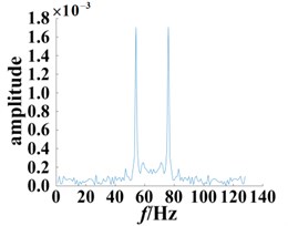
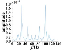
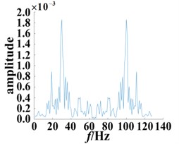
In practical applications, the influence of the device should be taken into account. Based on the experimental results, the external noise based on different signal-to-noise ratios, SNR = 12 dB and SNR = 6 dB, were added to the collected signals to simulate the effect of smooth operation and non-stationary operation. Using the method developed in this paper, the data was analyzed and used to produce the bispectrum based on the Volterra kernel function, as shown in Fig. 10. This was then compared to the experimental results.

Fig. 10Slices of bispectrum based on the second-order kernel (SNR = 12 dB)

a) Normal bearing

b) Damaged bearing with 0.18 mm diameter fault

c) Damaged bearing with 0.36 mm diameter fault

Comparing Figs. 9 and 10, it is found that after adding the external noise with SNR = 12 dB, although some fluctuations appear, the frequency points corresponding to its peak are not affected as a whole. The bispectrum slices of the normal bearing still show the highest peaks at $f=$56 Hz and $f=$ 77 Hz. Similarly, the bearing bispectral slices for the damage diameter of 0.18 mm have peaks at $f=$ 28 Hz, $f=$ 46 Hz, $f=$ 57 Hz, $f=$ 75 Hz, $f=$ 83 Hz, $f=$ 101 Hz, and other significant peaks also appear nearby. For the 0.36 mm diameter fault, the bispectrum slice distribution of the bearing is more dispersed, and there are significant peaks at $f=$ 14 Hz, $f=$ 19 Hz, $f=$ 28 Hz, $f=$ 47 Hz, $f=$ 58 Hz, $f=$ 74 Hz, $f=$ 83 Hz, $f=$ 102 Hz and $f=$ 113 Hz. The different secondary phase coupling phenomena can be described and compared by the different degrees of damage to the fault bearing.

When external noise was present, the signal-to-noise ratio SNR = 6 dB was added, and the bispectrums for the different degrees of damage were produced. The peak arrangement was disorderly, and the useful information was hidden by noise; therefore, it was difficult to extract the fault features. More detailed information can be derived from the 3rd order and above for the higher order Volterra kernel function, however we do not elaborate on this here. In general, the results of the analysis, with either no external noise or adding a certain SNR based on the external noise, are consistent. The influence of external conditions can cause clutter in the signal, however the secondary coupling frequency point position does not have much impact. Under these conditions, the equipment has no obvious shock, and the method can ignore the influence of some of the equipment itself, and can therefore be applied to determine the faulty bearing characteristics due to different degrees of damage.

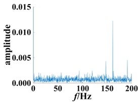
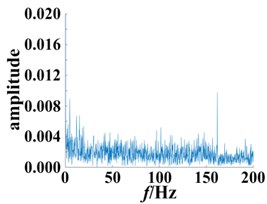
The wavelet and envelope method was used to analyze the bearing under the same experimental conditions. After adding the external noise (SNR = 12 dB), the output signal was subjected to the wavelet, denoting the envelope analysis, and compared with the proposed methods in this paper. The roller fault characteristic frequency can be defined as:

25

$f_{inner}=\frac{z}{2}\left(1+\frac{d}{D}\mathrm{c}\mathrm{o}\mathrm{s}\alpha \right)\frac{n}{60}.$

Using the data obtained in the experiment, this was calculated as $f_{inner}=$ 159.7 Hz.

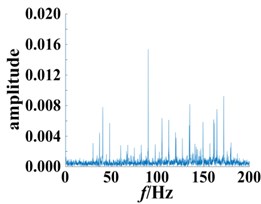
The wavelet base was chosen as “db6” and subjected to the Hilbert envelope analysis, as shown in Fig. 11, and compared to the multi-pulse excitation method described above.

The envelope spectrum of the normal bearing was compared to bearings with different degrees of damage, as shown in Fig. 11. The frequency point of the highest peak was at 161.2 Hz. (Fig. 11(b-c)), which is consistent with the theoretically calculated fault frequency point. Building upon these results, the frequency point can be used to distinguish the normal bearing and roller fault bearing. A shown in Fig. 11(b) and 11(c), with the exception of the peak (161.2 Hz), the rest of the fluctuations also increased as the degree of the fault increased. However, its distribution is irregular, making it difficult to extract additional fault information. A significant advantage of the method presented in this paper is the use of Volterra series modeling together with the secondary phase coupling frequency, represented by the second order kernel function bispectrum slice figure to show the fault features. This can be used to assess the different degrees of damage to a bearing. In addition, bispectrum analysis is insensitive to noise, so it can continue to extract the characteristics of the bearing provided there is no obvious impact, and thus to a certain extent, overcome the influence of the equipment itself.

Fig. 11Envelope spectrum based on different degrees of bearing damage

a) Normal bearing

b) Bearing with 0.18 mm diameter fault

c) Bearing with 0.36 mm diameter fault

7. Conclusions

The Volterra series can be used to extract weak faults in nonlinear systems. Using low-order nuclei, the Volterra series was obtained using the multi-pulse excitation method, identified by the second-order and third-order nuclei of the GIRF and GFRF. The proposed method can more easily extract the fault characteristics of a non-linear system compared to the traditional wavelet transform method. It was found that the multi-pulse excitation method has its own unique characteristics. The method is relatively straight-forward and can simplify the filtering and selection of the wavelet for analysis. The wavelet system is very complicated, however the input and output of the system can be used to assess and extract the fault characteristics, which can then be used to determine the transfer function of the system, while neglecting any interference from the outside world.