Two-dimensional generalized thermo-elastic problem for anisotropic half-space

Ghosh, Debkumar; Lahiri, Abhijit; A. Abbas, Ibrahim

doi:10.21595/mme.2017.18236

Mathematical Models in Engineering

Browse Journal

Submit article

Published: 30 June 2017

Check for updates

Two-dimensional generalized thermo-elastic problem for anisotropic half-space

Debkumar Ghosh¹

Abhijit Lahiri²

Ibrahim A. Abbas³

^{1, 2}Department of Mathematics, Jadavpur University, Kolkata, 700032, India

³Department of Mathematics, Sohag University, Sohag, Egypt

Corresponding Author:

Debkumar Ghosh

Cite the article Download PDF

Downloads 1541

CrossRef Citations 3

Abstract

This paper concerns with the study of wave propagation in fibre reinforced anisotropic half space under the influence of temperature and hydrostatic initial stress. Lord-Shulman theory is applied to the heat conduction equation. The resulting equations are written in the form of vector matrix differential equation by using Normal Mode technique, finally which is solved by Eigen value approach.

1. Introduction

Fibre-reinforced composite(FRC) materials are usually low weight and high strength used in construction engineering. The physical property of FRC material is governed by the theory of elasticity for different materials with the direction along the direction of fibre. Green [1] studied wave propagation in anisotropic elastic plates. Abbas and Othman [2] discussed the distribution of wave propagation under hydrostatic initial stress of fibre-reinforced materials in anisotropic half-space. Baylies and Green [3] analyse the flexural waves in fibre-reinforced laminated plates. Rogerson [4] discussed effect of penetration in a six-ply composite laminates.

Most of the thermoelasticity and generalized thermoelasticity (coupled or uncoupled) problems have been solved by potential function approach. This method is not always suitable as discussed by Dhaliwal and Sherief [5] and Sherief and Anwar [6]. These may be summarized by the initial conditions and the boundary conditions for physical problems which are directly concern with the material quantities under consideration and not with the potential function. Also, the potential function representations are not convergent always while the physical problems in natural variables constitute convergent solution. So, the alternative method of potential function approach is eigenvalue approach. In this method, we obtain a vector-matrix differential equation from the basic equations which reduces finally to an algebraic eigenvalue problem and the solutions for the field variables are obtained by determining the eigenvalues and eigenvectors from the corresponding coefficient matrix. In this theory, body forces and/or heat sources are also accommodated as in Das and Lahiri [7], Bachher et al. [8]. Now, two different models of generalized thermoelastisities are extensively used. One is Lord and Shulman (L-S) [9] theory and the other is Green and Lindsay (G-L) [10] theory. Introducing one relaxtion time parameter in L-S theory the heat conduction equation becomes hyperbolic type without violating conventional Fourier’s law. Whereas the G-L theory modified the heat conduction equation as well as the equation of motion in coupled thermoelasticitywo relaxation time parameters. There are other three models (Model I, II and III by Green and Nagdhi [11-13]) for generalized thermoelasticity concerned to the theory of with or without energy dissipation.

2. Development of governing equations

The stress-strain relation and the governing equations of motion without body forces and heat sources are written as follow:

1

σ_{i j, j} - P ω_{i j, j} = ρ {\ddot{u}}_{i},

2

σ_{i j} = λ e_{k k} δ_{i j} + 2 μ_{T} e_{i j} + α (a_{k} a_{m} e_{k m} δ_{i j} + a_{i} a_{j} e_{k k})

+ 2 (μ_{L} - μ_{T}) (a_{i} a_{k} e_{k j} + a_{j} a_{k} e_{k i}) + β a_{k} a_{m} e_{k m} a_{i} a_{j} - β_{i j} (T - T_{0}) δ_{i j}, i, j, k, m = 1,2, 3,

3

e_{i j} = \frac{1}{2} (u_{i, j} + u_{j, i}),

4

ω_{i j} = \frac{1}{2} (u_{j, i} - u_{i, j}),

5

K_{i j} T_{i j} = ρ c_{e} (\dot{T} + t_{0} \ddot{T}) + T_{0} ({\dot{u}}_{i, j} {\ddot{u}}_{i, j}), i, j = 1,2, 3 .

We consider the problem of a elastic half-space $(x \geq 0)$ in fibre-reinforced anisotropic material with $a \equiv (a_{1}, a_{2}, a_{3})$ where $a_{1}^{2} + a_{2}^{2} + a_{3}^{2} = 1$ as in I. A. Abbas [14], where the displacements are given:

6

u = u_{x} = u (x, y, t), v = u_{y} = v (x, y, t), w = u_{z} = 0 .

We consider the direction of fibre as $a \equiv (1,0, 0)$ with $x$ -axis as prefered direction, and Eqs. (1-5), reduces as given:

7

σ_{11} = (λ + 2 α + 4 μ_{L} - 2 μ_{T} + β) \frac{\partial u}{\partial x} + (λ + α) \frac{\partial v}{\partial y} - β_{11} (T - T_{0}),

8

σ_{22} = (λ + 2 μ_{T}) \frac{\partial v}{\partial y} + (α + λ) \frac{\partial u}{\partial x} - β_{22} (T - T_{0}),

9

σ_{12} = μ_{L} (\frac{\partial v}{\partial x} + \frac{\partial u}{\partial y}),

10

A_{11} \frac{\partial^{2} u}{\partial x^{2}} + (A_{12} + μ_{L} - \frac{P}{2}) \frac{\partial^{2} v}{\partial x \partial y} + (μ_{L} + \frac{P}{2}) \frac{\partial^{2} u}{\partial y^{2}} - β_{11} \frac{\partial T}{\partial x} = ρ \frac{\partial^{2} u}{\partial t^{2}},

11

A_{22} \frac{\partial^{2} v}{\partial y^{2}} + (A_{12} + μ_{L} - \frac{P}{2}) \frac{\partial^{2} u}{\partial x \partial y} + (μ_{L} + \frac{P}{2}) \frac{\partial^{2} v}{\partial x^{2}} - β_{22} \frac{\partial T}{\partial y} = ρ \frac{\partial^{2} v}{\partial t^{2}},

12

K_{11} \frac{\partial^{2} T}{\partial x^{2}} + K_{22} \frac{\partial^{2} T}{\partial y^{2}} = (\frac{\partial}{\partial t} + t_{0} \frac{\partial^{2}}{\partial t^{2}}) (ρ c_{e} T + T_{0} β_{11} \frac{\partial u}{\partial x} + T_{0} β_{22} \frac{\partial v}{\partial y}),

with:

A_{11} = λ + 2 (α + μ_{L}) + 4 (μ_{L} - μ_{T}) + β, A_{12} = α + λ, A_{22} = λ + 2 μ_{T},

β_{11} = (2 λ + 3 α + 4 μ_{L} - 2 μ_{T} + β) α_{11} + (λ + α) α_{22}, β_{22} = (2 λ + α) α_{11} + (λ + 2 μ_{T}) α_{22},

where $α_{11}$ , $α_{22}$ are linear thermal expansion coeeficients.

To transform the above governing equations in non-dimensional forms, we introduce the non-dimensional variables as follows:

13

(x^{'}, y^{'}, u^{'}, v^{'}) = c_{1} χ (x, y, u, v), t^{'} = c_{1}^{2} χ t, T^{'} = \frac{β_{11} (T - T_{0})}{ρ c_{1^{2}}}, χ = \frac{ρ c_{e}}{K_{11}},

({σ^{'}}_{11}, {σ^{'}}_{12}, {σ^{'}}_{22}) = \frac{1}{ρ c_{1}^{2}} (σ_{11}, σ_{12}, σ_{22}), c_{1}^{2} = \frac{A_{11}}{ρ} .

Using non-dimensional Eq. (13), the governing equations reduces to (eleminating primes for convenience):

14

σ_{11} = \frac{\partial u}{\partial x} + B_{1} \frac{\partial v}{\partial y} - T,

15

σ_{22} = B_{1} \frac{\partial u}{\partial x} + B_{2} \frac{\partial v}{\partial y} - B_{3} T,

16

σ_{12} = B_{4} (\frac{\partial v}{\partial x} + \frac{\partial u}{\partial y}),

17

\frac{\partial^{2} u}{\partial x^{2}} + (B_{1} + B_{4} - \frac{R_{p}}{2}) \frac{\partial^{2} v}{\partial x \partial y} + (B_{4} + \frac{R_{p}}{2}) \frac{\partial^{2} u}{\partial y^{2}} - \frac{\partial T}{\partial x} = \frac{\partial^{2} u}{\partial t^{2}},

18

B_{2} \frac{\partial^{2} v}{\partial y^{2}} + (B_{1} + B_{4} - \frac{R_{p}}{2}) \frac{\partial^{2} u}{\partial x \partial y} + (B_{4} + \frac{R_{p}}{2}) \frac{\partial^{2} v}{\partial x^{2}} - B_{3} \frac{\partial T}{\partial y} = \frac{\partial^{2} v}{\partial t^{2}},

19

\frac{\partial^{2} T}{\partial x^{2}} + ε_{1} \frac{\partial^{2} T}{\partial y^{2}} = (\frac{\partial}{\partial t} + t_{0} \frac{\partial^{2}}{\partial t^{2}}) (T + ε_{2} \frac{\partial u}{\partial x} + ε_{3} \frac{\partial v}{\partial y}),

where:

(B_{1}, B_{2}, B_{3}) = \frac{1}{A_{11}} (A_{12}, A_{22}, μ_{1}), B_{3} = \frac{β_{22}}{β_{11}}, R_{p} = \frac{P}{A_{11}},

(ε_{2}, ε_{3}) = \frac{T_{0} β_{11}}{A_{11} ρ c_{e}} (β_{11}, β_{22}), ε_{1} = \frac{K_{11}}{K_{22}} .

3. Solution procedure

3.1. Normal mode analysis: formulation of vector-matrix differential equation

For the solution of the Eqs. (14-19), physical variables can be decomposed using normal modes Eq. (20) in the following form:

20

[u, v, T, σ_{11}, σ_{12}, σ_{22}] (x, y, t) = [u^{*}, v^{*}, T^{*}, σ_{11}^{*}, σ_{12}^{*}, σ_{22}^{*}] (x) e^{ω t + i a y},

where $i = \sqrt{- 1}$ , $ω$ is the angular frequency and a is the wave number along $x$ -axis.

Using Eq. (20), Eqs. (14-19) reduces to omitting ‘*’ for convenience:

21

σ_{11} = \frac{d u}{d x} + (B_{1} i a) v - T,

22

σ_{22} = B_{1} \frac{d u}{d x} + (B_{2} i a) v - B_{3} T,

23

σ_{12} = B_{4} \frac{d v}{d x} + (B_{4} i a) u,

24

\frac{d^{2} u}{d x^{2}} = M 41 . u + 0 . v + 0 . T + 0 . u^{'} + M 45 . v^{'} + T^{'},

25

\frac{d^{2} v}{d x^{2}} = 0 . u + M 52 . v + M 53 . T + M 54 . u^{'} + 0 . v^{'} + 0 . T^{'},

26

\frac{d^{2} T}{d x^{2}} = 0 . u + M 62 . v + M 63 . T + M 64 . u^{'} + 0 . v^{'} + 0 . T^{'},

where:

M 41 = a^{2} [B_{4} + \frac{R_{p}}{2}] + ω^{2}, M 45 = - i a [B_{1} + B_{4} - \frac{R_{p}}{2}], M 52 = \frac{a^{2} B_{2} + ω^{2}}{B_{4} + \frac{R_{p}}{2}},

M 53 = \frac{\frac{R_{p}}{2} - B_{1} - B_{4}}{B_{4} + \frac{R_{p}}{2}}, M 54 = \frac{i a B_{3}}{B_{4} + \frac{R_{p}}{2}}, M 62 = i a ε_{3} (ω + t_{0} ω^{2}),

M 63 = ω + t_{0} ω^{2} + ε_{2} a^{2}, M 64 = ε_{2}^{2} (ω + t_{0} ω^{2}) .

Eqs. (24-26) can be written in the form of vector-matrix differential equation as [2, 8]:

27

\frac{d \vec{W}}{d x} = \vec{A} \vec{W},

where $\vec{W}$ = ${[u v T u^{'} v^{'} T^{'}]}^{T}$ and $A = [\begin{array}{l} L_{11} & L_{12} \\ L_{21} & L_{22} \end{array}]$ . Where $L_{11}$ is null matrix and $L_{12}$ identity matrix of order 3×3 respectively and $L_{21}$ and $L_{22}$ are given by:

L_{11} = (\begin{array}{l} 0 & 0 & 0 \\ 0 & 0 & 0 \\ 0 & 0 & 0 \end{array}), L_{12} = (\begin{array}{l} 1 & 0 & 0 \\ 0 & 1 & 0 \\ 0 & 0 & 1 \end{array}),

L_{21} = (\begin{matrix} M 41 & 0 & 0 \\ 0 & M 52 & M 53 \\ 0 & M 62 & M 63 \end{matrix}), L_{22} = (\begin{matrix} 0 & M 45 & 1 \\ M 54 & 0 & 0 \\ M 64 & 0 & 0 \end{matrix}) .

3.2. Solution of the vector-matrix differential equation

To solve the vector-matrix differential Eq. (27), we apply the method of eigenvalue approach,

The characteristic equation of the matrix $\vec{A}$ is given by:

28

|A - λ I| = 0 .

The roots of the characteristic Eq. (28) are $λ = λ_{i}$ , $i =$ 1, 2, 3 which are of the form $λ = \pm λ_{1}$ , $λ = \pm λ_{2}$ and $λ = \pm λ_{3}$ and they are also eigenvalues of the matrix.

The eigenvector, $\vec{W}$ corresponding to the eigenvalue $λ$ can obtained as:

29

{\vec{X}}_{λ} = {[δ_{1} δ_{2} δ_{3} λ δ_{1} λ δ_{2} λ δ_{3}]}^{T},

where $δ_{1} = a_{2} b_{3} - a_{3} b_{2}$ , $δ_{2} = a_{3} b_{1} - a_{1} b_{3}$ , $δ_{3} = a_{1} b_{2} - a_{2} b_{1}$ .

As in Lahiri et al. [7], the general solution of Eq. (27) which is regular as can be written as:

30

\vec{W} = \sum_{i = 1}^{3} ‍ A_{i} X_{i} e^{- λ_{i} x}, x \geq 0 .

Hence the field variables can be written as the following:

u = A_{1} x_{11} e^{- λ_{1} x} + A_{2} x_{21} e^{- λ_{2} x} + A_{3} x_{31} e^{- λ_{3} x},

v = A_{1} x_{12} e^{- λ_{1} x} + A_{2} x_{22} e^{- λ_{2} x} + A_{3} x_{32} e^{- λ_{3} x},

T = A_{1} x_{13} e^{- λ_{1} x} + A_{2} x_{23} e^{- λ_{2} x} + A_{3} x_{33} e^{- λ_{3} x} .

The simplified form of Eqs. (21-23) can be written as:

\begin{array}{l} σ_{11} = A_{1} R_{11} (x) + A_{2} R_{12} (x) + A_{3} R_{13} (x), \\ σ_{22} = A_{1} R_{21} (x) + A_{2} R_{22} (x) + A_{3} R_{23} (x), \\ σ_{33} = A_{1} R_{31} (x) + A_{2} R_{32} (x) + A_{3} R_{33} (x), \end{array}

where:

R_{11} (x) = [- λ_{1} x_{11} + B_{1} i a x_{12} - x_{13}] e^{- λ_{1} x},

R_{12} (x) = [- λ_{2} x_{21} + B_{1} i a x_{22} - x_{23}] e^{- λ_{2} x},

R_{13} (x) = [- λ_{3} x_{31} + B_{1} i a x_{32} - x_{33}] e^{- λ_{3} x},

R_{21} (x) = [- λ_{1} B_{1} x_{11} + B_{2} i a x_{12} - B_{3} x_{13}] e^{- λ_{1} x},

R_{21} (x) = [- λ_{2} B_{1} x_{21} + B_{2} i a x_{22} - B_{3} x_{23}] e^{- λ_{2} x},

R_{21} (x) = [- λ_{3} B_{1} x_{31} + B_{2} i a x_{32} - B_{3} x_{33}] e^{- λ_{3} x},

R_{31} (x) = [B_{4} i a x_{11} - λ_{1} x_{12}] e^{- λ_{1} x},

R_{32} (x) = [B_{4} i a x_{21} - λ_{2} x_{22}] e^{- λ_{2} x},

R_{33} (x) = [B_{4} i a x_{31} - λ_{3} x_{32}] e^{- λ_{3} x} .

4. Boundary conditions

Considering the problem of a half-space $ϕ$ , defined as follows:

ϕ = (x, y, z) : 0 \leq x \leq \infty, - \infty \leq y \leq \infty, - \infty \leq z \leq \infty .

In order to determine the arbitrary constants $A_{i}^{'} s$ , $i =$ 1, 2, 3, we consider the boundary conditions as follows.

4.1. Case 1

a) Mechanical Boundary condition:

For stress-free surface $x =$ 0, $σ_{11} = 0$ , $σ_{12} = 0 .$

b) Thermal Boundary condition:

31

ν T - \frac{d T}{d x} = r,

where $ν$ is Biot’s number.

4.2. Case 2

a) Mechanical Boundary condition:

For stress-free surface $x =$ 0, $σ_{11} = - P_{1} + P_{2} e^{ω t + i a y}$ , $σ_{12} = 0$ .

b) Thermal Boundary condition:

32

T = P_{3} e^{ω t + i a y} .

5. Numerical analysis

5.1. Case 1

5.1.1. Distribution of different stress components

Fig. 1 represents distribution of normal stress $σ_{11}$ for $y =$ 0.3.

For fixed time $t$ , $σ_{11}$ gradually increases as $x$ increases. For fixed $x$ numerical values of $σ_{11}$ gradually decreases as t increases.

Fig. 2 represents distribution of normal stress $σ_{12}$ for $y =$ 0.2.

For fixed time $t$ , $σ_{12}$ gradually decreases as $x$ increases. For fixed x numerical values of $σ_{12}$ gradually increases as $t$ increases.

Fig. 3 represents distribution of normal stress $σ_{22}$ for $y =$ 0.5.

For fixed time $t$ , $σ_{22}$ gradually decreases as $x$ increases. For fixed $x$ numerical values of $σ_{12}$ gradually increases as $t$ increases.

Fig. 1Stress component σ11 at y= 0.3 for different values of t verses x

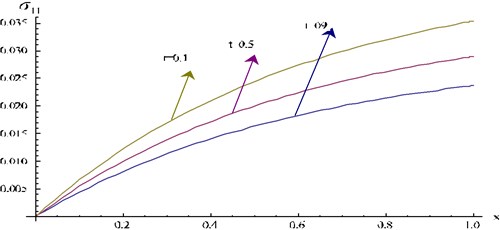
Fig. 2Stress component σ12 at y= 0.2 for different values of t verses x

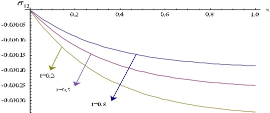
Fig. 4 represents distribution of normal stress $σ_{11}$ for different values of $x$ and $y$ for fixed $t =$ 0.1 and $ω =$ 0.5.

$x$ numerical value of $σ_{11}$ gradually decreases as $y$ increases. For fixed $y$ the numerical value of $σ_{11}$ gradually increases as $x$ increases. $σ_{11}$ is maximum when $x =$ 1 and $y =$ 0.

Fig. 5 represent distribution of normal stress $σ_{12}$ for different values of $x$ and $y$ for fixed $t =$ 0.4 and $ω =$ 5.

For fixed $x$ numerical value of $σ_{12}$ gradually decreases as $y$ increases. For fixed $y$ the numerical value of $σ_{12}$ gradually decreases as $x$ increases. Significant changes occur in the region 0.2 $\leq x \leq$ 0.6 and 0.6 $\leq y \leq$ 1.0.

Fig. 6 represent distribution of stress component $σ_{22}$ at for different values of $x$ and $y$ for fixed $t =$ 0.1 and 0.1.

Fig. 4Stress component σ11 at t= 0.1 and ω= 0.5 verses x and y

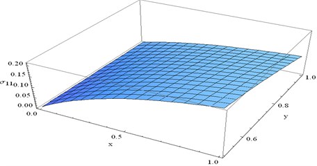
Fig. 5The variation of stress component σ12 at t= 0.4 and ω= 3 verses x and y

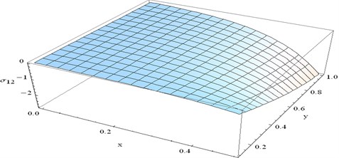
Fig. 6Stress component σ22 at t= 0.1 and ω= 0.1 verses x and y

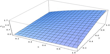
For fixed $x$ numerical value of $σ_{22}$ gradually increases as $y$ increases. For fixed $y$ numerical value of $σ_{22}$ gradually increases as $x$ increases.

Fig. 7 represent distribution of normal stress $σ_{12}$ for different values of $x$ and $t$ for fixed $y =$ 0.2 and 1.

For fixed $x$ , nominal decreasing of numerical values of $σ_{12}$ has been seen as $t$ increases, while For fixed $t$ , numerical values of $σ_{12}$ decreases gradually as $x$ increases. numerical values of $σ_{12}$ minimum at $x =$ 1 and 0.02 $\leq t \leq$ 0.1

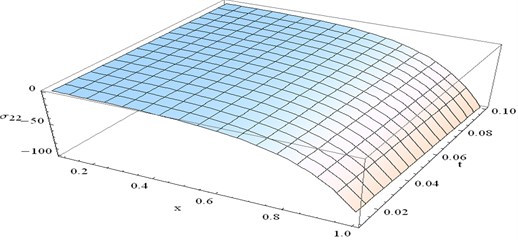
Fig. 8 represent distribution of normal stress $σ_{22}$ for different values of $x$ and $t$ for fixed $y =$ 0.5 and 2.

For fixed $x$ , nominal decreasing of $σ_{22}$ has been seen as t increases. For fixed $t$ , numerical values of $σ_{12}$ decreases as $x$ increases. Also, significant changes occur in the region 0.6 $\leq x \leq$ 1.0 and 0 $\leq t \leq$ 1.0.

Fig. 7Stress component σ12 at y= 0.2 and ω= 1 verses x and t

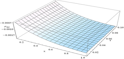
Fig. 8The distribution of stress component σ22 at y= 0.5 and ω= 2 verses x and t

5.1.2. Distribution of temperature

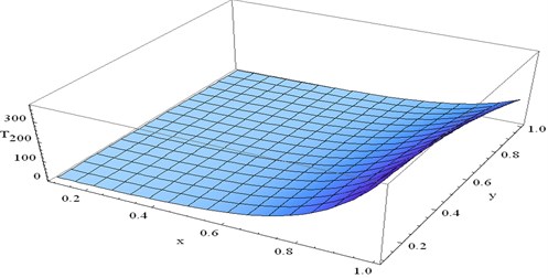
Fig. 9 represent distribution of temperature, $T$ for different values of $x$ and $y$ for fixed $t =$ 0.3 and 2.

For fixed $x$ numerical value of $T$ gradually decreases as $y$ increases. For fixed $y$ numerical value of $T$ gradually increases as $x$ increases. $T$ in minimum at $x =$ 0 and significant changes occurs in the region 0.6 $\leq x \leq$ 1.0 and 0 $\leq y \leq$ 1.0

Fig. 10 represent distribution of temperature, $T$ for different values of $x$ and $t$ for fixed $y =$ 0.1 and 1.5.

Fig. 9The variation of T at t= 0.3 and ω= 2 verses x and y

For fixed $t$ numerical value of $T$ nominally increases as $x$ increases. For fixed $x$ numerical value of $T$ gradually increases as $t$ increases.

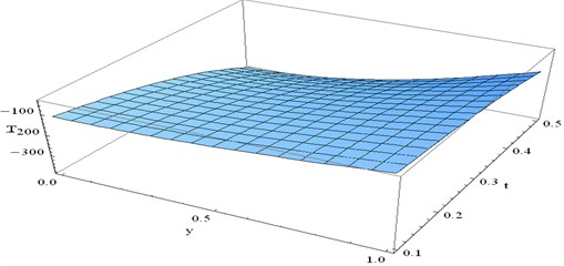
Fig. 11 represent distribution of temperature, $T$ for different values of $y$ and $t$ for fixed $x =$ 0.5 and 3.

For fixed $t$ numerical value of $T$ nominally increases as $y$ increases. For fixed $x$ numerical values of $T$ decreases as $t$ increases.

Fig. 10Variation of T at y= 0.1 and ω= 1.5 verses x and t

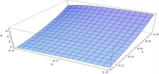
Fig. 11Variation of T at x= 0.5 and ω= 3 verses y and t

5.2. Case 2

5.2.1. Distribution of different stress components

Fig. 12 represents distribution of normal stress $σ_{11}$ for $y =$ 0.3, $t =$ 0.01 and 5 for different numerical values of $R_{p}$ .

For fixed $R_{p}$ , $σ_{11}$ gradually decreases as $x$ increases. For fixed x numerical values of $σ_{11}$ gradually decreases as $R_{p}$ increases.

Fig. 13 represents distribution of normal stress $σ_{11}$ for $y =$ 0.3, $t =$ 0.01 and 5 for different fractional values of $R_{p}$ .

For fixed time $R_{p}$ , $σ_{11}$ gradually increases as $x$ increases. For fixed $x$ numerical values of $σ_{11}$ gradually decreases as $R_{p}$ increases. Significant changes occurred for 0 $\leq x \leq$ 0.4.

Fig. 14 represents the distribution of stress component $σ_{12}$ at $y =$ 0.2, $t =$ 0.03 and 0.3 for different fractional values $R_{p}$ of verses $x$ for $P 1 =$ 1.

For fixed time $R_{p}$ , $σ_{11}$ gradually decreases as $x$ increases. For fixed x numerical values of $σ_{11}$ increases as $R_{p}$ increases. Significant changes occurred for 0 $\leq x \leq$ 0.4.

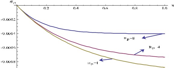
Fig. 15 represents the distribution of stress component $σ_{12}$ at $y =$ 0.3, $t =$ 0.1 and 4 for different integral values $R_{p}$ for $P 1 =$ 0.

For fixed $R p$ , $σ_{12}$ gradually decreases as $x$ increases. For fixed $x$ numerical values of $σ_{12}$ increases as $R_{p}$ increases.

Fig. 16 represents the distribution of stress component $σ_{22}$ at $y =$ 0.2, $t =$ 0.6 and 0.4 for different values $R_{p}$ for $P 1 =$ 0.

For fixed $R_{p} =$ 0.9, $σ_{22}$ gradually increases as $x$ increases but for other fixed values of $R_{p}$ , $σ_{22}$ gradually decreases as $x$ increases. For fixed $x$ , $σ_{22}$ gradually increases as $x$ increases for $R_{p} =$ 0.9 but for other fixed values of $R_{p}$ , $σ_{22}$ gradually decreases as $x$ increases.

Fig. 17 represents the distribution of stress component $σ_{11}$ for different values of $t$ for fixed $y =$ 0.2 and 1.5.

Fig. 12Stress component σ11 at y= 0.3, t= 0.01 and ω= 5 for different values Rp of verses x

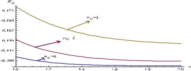
Fig. 13Stress component σ11 at y= 0.2 and ω= 0.2 for different values Rp of verses x

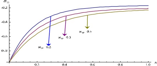
Fig. 14Stress component σ12 at y= 0.2, t= 0.03 and ω= 0.3 for different values Rp of verses x for P1= 1

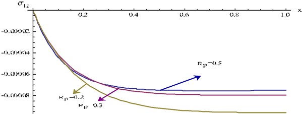
Fig. 15Stress component σ12 at y= 0.3, t= 0.1 and ω= 4 for different values Rp of verses x for P1= 0

For fixed $t$ , the numerical value of $σ_{11}$ gradually increases as $x$ increases. For fixed $x$ , the numerical value of $σ_{11}$ gradually increases as $t$ increases.

Fig. 18 The distribution of stress component $σ_{12}$ for fixed $y =$ 0.3 and 0.5 for different values of $t$ .

For fixed $t$ , the numerical value of $σ_{12}$ gradually decreases as $x$ increases. For fixed $x$ , the numerical value of $σ_{12}$ gradually increases as $t$ increases.

Fig. 16Stress component σ22 at y= 0.2, t= 0.6 and ω= 0.4 for different values Rp of verses x for P1= 0

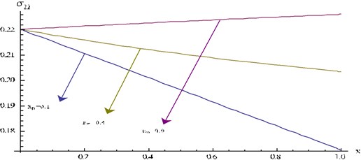
Fig. 17Stress component σ11 at y= 0.2 and ω= 1.5 for different values of t verses x

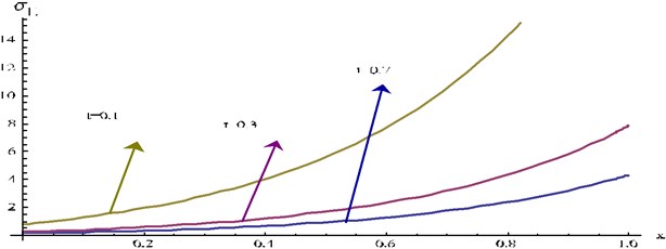
Fig. 18Stress component σ12 at y= 0.3 and ω= 0.5 for different values of t verses x

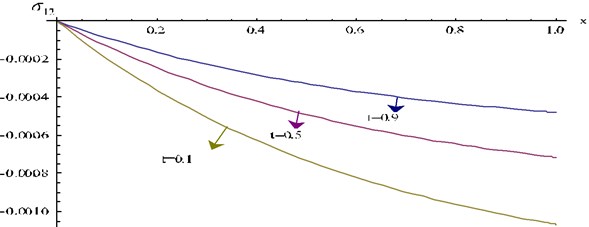
Fig. 19Stress component σ22 at y= 0.5 and ω= 0.2 for different values of t verses x

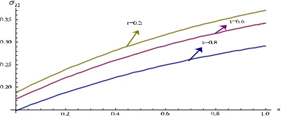
Fig. 19 represents the distribution of stress component $σ_{22}$ at fixed $y =$ 0.5 and 0.2 for different values of $t$ .

For fixed $t$ , the numerical value of $σ_{12}$ gradually increases as $x$ increases, but for fixed $x$ , the numerical value of $σ_{12}$ gradually decreases as t increases.

Fig. 20 represents distribution of normal stress $σ_{11}$ for different values of $x$ and for fixed $t =$ 0.3 and $y =$ 0.3.

For fixed $x$ numerical value of $σ_{11}$ remain constant as increases, but for fixed $ω$ the numerical value of $σ_{11}$ gradually decreases as $x$ increases.

Fig. 21 represents distribution of normal stress $σ_{12}$ for different values of $x$ and for fixed $y =$ 0.3 and $t =$ 0.5.

For fixed $x$ , nominal increasing of numerical values of $σ_{12}$ has been seen as increases, while for fixed $ω$ , numerical values of $σ_{12}$ increases gradually as $x$ increases after $x =$ 0.6 (approx.). Numerical values of $σ_{12}$ minimum at $x =$ 0.5 (approx.) and 1 $\leq t \leq$ 3.

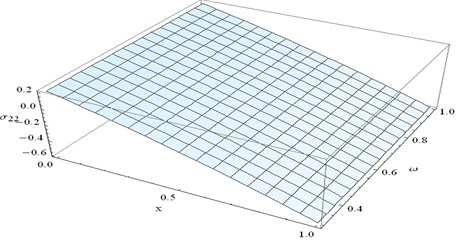
Fig. 22 represents distribution of stress component $σ_{22}$ at for different values of $x$ and for fixed $t =$ 0.1 and $y =$ 0.4.

For fixed $ω$ numerical value of $σ_{22}$ gradually decreases as $x$ increases. Numerical values of $σ_{22}$ minimum at $x =$ 1 and 0 $\leq ω \leq$ 1.

Fig. 20Stress component σ11 at y= 0.3 and t= 0.3 verses x and ω

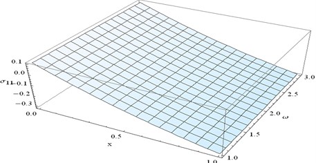
Fig. 21Stress component σ12 at y= 0.3 and t= 0.5 verses x and ω

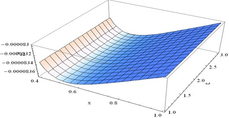
Fig. 22Stress component σ22 at y= 0.4 and t= 0.1 verses x and ω

5.2.2. Distribution of temperature

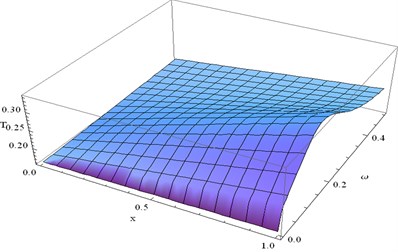
Fig. 23 represents distribution of temperature, $T$ for different values of $x$ and $ω$ for fixed $t =$ 0.1 and $y =$ 0.4.

For fixed $x$ numerical value of $T$ gradually increases in the region 0 $\leq ω \leq$ 0.3 (approx.) For fixed $ω$ numerical value of $T$ nominally increases as $x$ increases.

Fig. 23The variation of T at y=0.4 and t= 0.1 verses x and ω

6. Conclusion

We consider the physical parameters in SI units given in Dhaliwal and Singh following below to obtain the numerical result to observe the effect of wave propagation:

ρ = 2660 k g / m^{3}, λ = 5.65 \times 1 0^{10} N / m^{2},

μ_{T} = 2.46 \times 1 0^{10} N / m^{2}, μ_{L} = 5.66 \times 1 0^{10} N / m^{2},

α = - 1.28 \times 1 0^{10} N / m^{2}, β = 220.90 \times 1 0^{10} N / m^{2},

α_{11} = 0.017 \times 1 0^{- 4} d e g^{- 1}, α_{22} = 0.015 \times 1 0^{- 4} d e g^{- 1},

l = 0.5, T_{0} = 293 K, c_{e} = 0.787 \times 1 0^{3} J K g^{- 1} d e g^{- 1}

K_{11} = 0.0921 \times 1 0^{10} J m^{- 1} s^{- 1} d e g^{- 1}

K_{22} = 0.0963 \times 1 0^{10} J m^{- 1} s^{- 1} d e g^{- 1}

P_{1} = 0 o r 1, P_{2} = 0.1, P_{3} = 0.2 .

References

Green W. A. Bending waves in strongly anisotropic plates. Quarterly Journal of Mechanics and Applied Mathematics, Vol. 35, 1982, p. 485-507.

Publisher
Abbas I. A., Othman M. I. A. Generalized thermoelastic interaction in a fiber-reinforced anisotropic half-space under hydrostatic initial stress. Journal of Vibration Control, Vol. 18, Issue 2, 2011, p. 175-182.

Publisher
Baylis E. R., Green W. A. Flexural waves in fiber reinforced laminated plates. Journal of Sound and Vibration, Vol. 110, 1986, p. 1-26.

Publisher
Rogerson G. A. Penetration of impact waves in a six-ply fiber composite laminate. Journal of Sound and Vibration, Vol. 158, 1992, p. 105-120.

Publisher
Dhaliwal R. S., Sherief H. H. Generalized thermoelasticity for anisotropic media. Quarterly of Applied Mathematics, Vol. 33, 1980, p. 1-8.

Publisher
Sherief H. H., El-Sayed A., El-Latief A. Fractional order theory of thermoelasticity. International Journal of Solids and Structures, Vol. 47, 2010, p. 269-275.

Publisher
Santra S., Das N. C., Kumar R., Lahir A. Three dimensional fractional order generalized thermoelastic problem under effect of rotation in a half space. Journal of Thermal Stresses, Vol. 38, 2015, p. 309-324.

Publisher
Bachher M., Sarkar N., Lahiri A. Generalized thermoelastic infinite medium with voids subjected to a instantaneous heat sources with fractional derivative heat transfer. International Journal of Mechanical Sciences, Vol. 89, 2014, p. 84-91.

Publisher
Lord H. W., Shulman Y. A generalized dynamical theory of thermoelasticity. Journal of the Mechanics and Physics of Solids, Vol. 15, 1967, p. 299-309.

Publisher
Green A. E., Lindsay K. A. Thermoelasticity. Journal of Elasticity, Vol. 2, 1972, p. 1-7.

Publisher
Green A. E., Naghdi P. M. A re-examination of the basic results of thermomechanics. Proceedings of the Royal Society of London A, Vol. 432, 1991, p. 171-194.

Publisher
Green A. E., Naghdi P. M. On undamped heat waves in an elastic solid. Thermal Stresses, Vol. 15, 1992, p. 252-264.

Publisher
Green A. E., Naghdi P. M. Thermoelasticity without energy dissipation. Elasticity, Vol. 31, 1993, p. 189-208.

Publisher
Ibrahim A. Abbas Generalized magnetothermoelasticity in a fiber-reinforced anisotropic half-space. International Journal of Thermophysics, 2011, https://doi.org/10.1007/s10765-011-0957-3.

Publisher

Cited by

Thermoelastic Interactions in a Microstretch Saturated Porous Medium with Temperature Dependent Properties

Amit Jangra | Sunita Deswal | Parmender Sheokand

(2024)

Modeling of a homogeneous isotropic half space in the context of multi-phase lag coupled thermoelasticity

Abhijit Lahiri | Sumit Sovan Sardar | Debkumar Ghosh

(2024)

The novel boundary integral equation with adaptive orthogonal IMLS based line integration method for cracked domains under thermal stress

Biao Liu | Wei Zhou | Qiao Wang

(2020)

About this article

Received

08 February 2017

Accepted

12 March 2017

Published

30 June 2017

DOI

https://doi.org/10.21595/mme.2017.18236

Keywords

eigenvalue

generalized thermoelasticity

normal mode

vector-matrix differential equation

This is an open access article distributed under the Creative Commons Attribution License, which permits unrestricted use, distribution, and reproduction in any medium, provided the original work is properly cited.

Previous article in issue Previous Next article in issue Next

Research article

2023 12 23

Plane waves in an isotropic thermoelastic diffusive material using strain gradient theory

Baljeet Singh, Himanshu Singla

Research article

2022 11 03

Eigen value approach with memory dependant derivative on homogeneous isotropic infinitely extended rotating plate of a finite thickness in absence of heat source

S. Chakraborty, A. Lahiri, B. Das

Research article

2019 09 30

Thermal shock behaviour on generalized thermoelastic semi-infinite medium with moving heat source under Green Naghdi-III model

Biswajit Singh, Smita Pal (Sarkar)

Research article

2017 06 30

Dynamic problem in 3D thermoelastic half-space with rotation in context of G-N type II and type III

S. Santra, A. Lahiri, N. C. Das

D. Ghosh, A. Lahiri, and I. A. Abbas, “Two-dimensional generalized thermo-elastic problem for anisotropic half-space,” Mathematical Models in Engineering, Vol. 3, No. 1, pp. 27–40, Jun. 2017, https://doi.org/10.21595/mme.2017.18236

Copy Extrica

Copied to clipboard!

TY  - JOUR
DO  - 10.21595/mme.2017.18236
UR  - https://doi.org/10.21595/mme.2017.18236
TI  - Two-dimensional generalized thermo-elastic problem for anisotropic half-space
T2  - Mathematical Models in Engineering
AU  - Ghosh, Debkumar
AU  - Lahiri, Abhijit
AU  - A. Abbas, Ibrahim
PY  - 2017
DA  - 2017/06/30
PB  - JVE International Ltd.
SP  - 27-40
IS  - 1
VL  - 3
SN  - 2351-5279
SN  - 2424-4627
ER  - 

Copy Ris

Copied to clipboard!

@article{Ghosh_2017,
	doi = {10.21595/mme.2017.18236},
	url = {https://doi.org/10.21595/mme.2017.18236},
	year = 2017,
	month = {jun},
	publisher = {{JVE} International Ltd.},
	volume = {3},
	number = {1},
	pages = {27--40},
	author = {Debkumar Ghosh and Abhijit Lahiri and Ibrahim A. Abbas},
	title = {Two-dimensional generalized thermo-elastic problem for anisotropic half-space},
	journal = {Mathematical Models in Engineering}
}

Copy Bibtex

Copied to clipboard!

[1]D. Ghosh, A. Lahiri, and I. A. Abbas, “Two-dimensional generalized thermo-elastic problem for anisotropic half-space,” Mathematical Models in Engineering, vol. 3, no. 1, pp. 27–40, Jun. 2017, doi: 10.21595/mme.2017.18236.

Copy IEEE

Copied to clipboard!

Ghosh, Debkumar, Abhijit Lahiri, and Ibrahim A. Abbas. “Two-Dimensional Generalized Thermo-Elastic Problem for Anisotropic Half-Space.” Mathematical Models in Engineering 3, no. 1 (June 30, 2017): 27–40. https://doi.org/10.21595/mme.2017.18236.

Copy Chicago

Copied to clipboard!

Two-dimensional generalized thermo-elastic problem for anisotropic half-space

Abstract

1. Introduction

2. Development of governing equations

3. Solution procedure

3.1. Normal mode analysis: formulation of vector-matrix differential equation

3.2. Solution of the vector-matrix differential equation

4. Boundary conditions

4.1. Case 1

4.2. Case 2

5. Numerical analysis

5.1. Case 1

5.1.1. Distribution of different stress components

5.1.2. Distribution of temperature

5.2. Case 2

5.2.1. Distribution of different stress components

5.2.2. Distribution of temperature

6. Conclusion

References

Cited by

About this article

Related Articles