Cantilever model with curvature nonlinearity and longitudinal inertia excited by lateral basal moments being Gaussian white noise

1. Introduction

Cantilever, as a kind of widely used basic structure, has drawn increasing interests in its dynamical problems in recent decades. In late years, response of cantilever subject to random excitation has arisen accelerating attention of researchers. The most prevalent method to study the structure vibration under random excitation is the stochastic finite element method (FEM). It is an effective numerical method that can directly obtain the response of the structures during simulation. Since the 1980s, this method has been widely employed and developed [1-4]. By now, compared with the numerical simulation methods i.e. FEM, theoretical model researches are far from abundant. Feng et al. [5-8]studied responses of cantilever model under narrow bounded noise excitation by the multi-time-scale method, the stochastic stability has been investigated, and the stochastic jumping phenomena has been observed. Koralek et al. [9] researched a atom force microscope cantilever excited by Gaussian white noise. Friswell et al. [10] analyzed responses of a randomly excited cantilever energy harvester. G. K. Er et al. [11] investigated a cantilever excited by lateral and axial excitations being Gaussian white noise, the model was treated as a multiple degree of freedom vibrating system and the probabilistic solutions were obtained by the state-space-split method. Those model researches about Gaussian white noise excitations seldom considered the nonlinear character, such as curvature nonlinearity and longitudinal inertia, induced by the geometrical deformation of the beam.

In this paper, a slender in-extensional cantilever model transversely excited by the Gaussian white noise at pedestal was studied. As well known, curvature nonlinearity [12, 13] and longitudinal inertia [14] have significant influence on the responses. Anderson and Nayfeh [12] studied the importance of the nonlinear curvature in the response of a cantilever under deterministic excitation experimentally and theoretically. In reference [13], stability analysis of axially oscillating cantilever beams excited by harmonic excitations were studied after considering the longitudinal inertia. In view of the fact that formal researches [9-11] who study the random vibrations usually focused on linear models, we concentrated on the model with curvature nonlinearity and inertia nonlinearity, and on the responses caused by the nonlinearity characters. Firstly, the inertia nonlinear term was expanded into Taylor series and the first two terms of them were kept. Then, the standard stochastic averaging method [15] was applied to simplify the system into two independent Ito functions of amplitude and phase, respectively. Subsequently, the stationary probability density function (PDF) of amplitude together with the joint PDF of the displacement and velocity were all given. After that, the reliability function and the probability density of the first passage failure time were studied theoretically and numerically. When the noise density is not too large, the theoretical approximations coincide with the digital results very well. While if noise density exceeds some certain threshold value, the theoretical approximation is less than perfect. One can find the theoretical results differ from the digital results slightly. Analysis showed that two main reasons lead to the error. One is the nonlinear stiffness term which will affect the response frequency, another is the truncation error happening during the Taylor series expanding. Finally, in section 5, a prediction-correction method was proposed to improve the performance of the theoretical predicting. Consequently, a new PDF of amplitude was obtained. After frequency variation induced by nonlinear stiffness was taken into account, numerical results verified the effectiveness of this modification.

2. Formulation

A well known dynamic model governing a slender in-extendable cantilever under basal transverse excitation was presented as follows [6-7, 16]. The deduction procedure was in the Appendix:

where $q\left(t\right)$ denotes the variable separated displacement function, $\varphi \left(s\right)$ denotes the module function:

where ${\lambda }_i$ are the roots of the character function$1+\mathrm{c}\mathrm{o}\mathrm{s}\left(\lambda \right)\mathrm{c}\mathrm{o}\mathrm{s}\mathrm{h}\left(\lambda \right)=$ 0, the first two of them are ${\lambda }_1=$ 1.8751, ${\lambda }_2=$ 4.6941. In this paper, we focus on the first module which is usually the most important. The transverse displacement of the cantilever is expressed as: $w(s,t)=q\left(t\right)\varphi \left(s\right)$. The beam was characterized by: the mass per unit length $m$, the bending stiffness $EI$, length $L$, and the acceleration of the transversal motion of the pedestal $z\left(t\right)$. The symbol $s$ denotes the axial Lagrange coordinate, ($\text{'}$) denotes partial derivative with respect to $s$, $(\cdot )$ denotes partial derivative with respect to time $t$.

Considering the linear damping $c\dot{w}$ and introducing the dimensionless transformation $\xi =s/L$, $y=q/L$, $\eta =z/L$, $\tau =t/T$, $T=\frac{1}{{\lambda }_1^2}\sqrt{m{L}^4/EI}$. The parameters are listed in the Table 1.

The dimensionless equation was obtained as:

where the coefficients are:

It is hypothesized that the basal transverse acceleration is the Gaussian white noise with zero mean, noise density $D$, and the correlation function $E\left[z\right(\tau \left)z\right(\tau +\mathrm{\Delta }\tau \left)\right]=D\delta \left(\mathrm{\Delta }\tau \right)$, where $\delta \left(\mathrm{\Delta }\tau \right)$ is the Dirac function.

As well known, the stochastic averaging method can be used in equations with the form of $\ddot{y}+g\left(y\right)+c(y,\dot{y})=f(y,\dot{y})\eta \left(t\right)$, which are called as the normalized equation, where $\ddot{y}$ is the inertia term, $g\left(y\right)$ is the stiffness term, $c(y,\dot{y})$ is the damping term, and $f(y,\dot{y})\eta \left(t\right)$ is the exciting term. But in Eq. (3), the inertia term is$({\alpha }_2{y}^2+1)\ddot{y}$, which is different from the normalized equation and may leave us some difficulties in applying stochastic averaging. The reason how this term turns out has been explicated in the appendix.

Then, Eq. (3) can be rewritten as:

Assuming the dimensionless displacement $y$ is smaller than 1, one can presume ${\alpha }_2{y}^2\ll 1$. For convenience, one can obtain $1/1+{\alpha }_2{y}^2\doteq 1-{\alpha }_2{y}^2$ by the Taylor series expanding. Substituting it into Eq. (4) and ignoring the nonlinear terms with order larger than 3, the Eq. (4) can be transformed to be:

Which is convenient for applying the stochastic averaging method.

Comparing the Eq. (5) with the governing motion equation in reference [11], it is obvious that we have the nonlinear stiffness term $({\alpha }_1-{\omega }_0^2{\alpha }_2)y^3$ and the nonlinear damping term ${\alpha }_{2}y{\dot{y}}^2(1-{\alpha }_2{y}^2)$, while the linear model in reference [11] doesn't have these mentioned terms. The effects of these nonlinear terms in narrowband noise excited equations have been illustrated in reference [6-8]. In the following section, we focus on the stochastic averaging method.

3. Standard stochastic averaging method

For convenience, the dimensionless time $\tau$ was still written as $t$ in the following text. At first, the coordinate transformation is introduced:

The premise of this transformation is that the influence of the nonlinear stiffness terms to the response frequency is weak enough. Thus, the response frequency can still be taken as ${\omega }_0$. The effectiveness of this assumption will be discussed and verified by numerical simulations later.

Substituting Eq. (6) into Eq. (5) yields:

where:

Applying the stochastic averaging [15] to Eq. (7), one obtains two independent Ito random differential equations about amplitude $A$ and phase $\phi$.

where $W_1\left(\tau \right)$, $W_2\left(\tau \right)$ denote standard Wiener process.

Compared with the phase, the interests are more focused on amplitude $A$. Then we take the amplitude $A$ in Eq. (8) as a one dimensional Markov process. The draft coefficient and the diffusion coefficient are:

The probability density of stationary response can be determined by Fokker-Planck-Kolmogorov equation (FPK):

The steady state solution of Eq. (12) can be got by letting $\partial p/\partial t=$ 0, then one get:

where $N$ is the normalization coefficient.

Substituting Eqs. (10), (11) into Eq. (13), the stationary probability density function of amplitude $A$ can be shows as follows:

The numerical simulation parameters were chosen as: non-dimensional linear damping coefficient $\mu =$ 0.3, noise density $D=$ 0.01, 0.02, 0.03 and 0.05 separately, time step $\mathrm{\Delta }t=$ 0.005, initial values $y\left(0\right)=\dot{y}\left(0\right)=$ 0, and other coefficients were seen in Eq. (3). Totally 5 000 sets of white noise of each noise density $D$ were imposed to the original system (3), each set of noise includes 30 000 numbers. The numerical solutions of the oscillator Eq. (3) could be obtained by an order-4 stochastic Runge-Kutta algorithm. The last 20 000 dots were kept as the steady state responses. The amplitude was taken as $A=\sqrt{y^2+{\dot{y}}^2/{\omega }_0^2}$. The steady states probability density function (PDF) of the amplitude were shown in Fig. 1.

Fig. 1Stationary PDF of amplitude (solid lines: theoretical approximation; dots: numerical simulation)

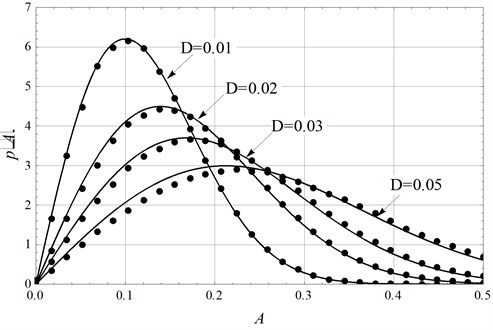
The solid lines in Fig. 1 present the analytical solution given by Eq. (14), the dots are obtained by numerical simulations. With noise density $D$ increasing from 0.01 to 0.03, the theoretical approximations coincide with the simulation results very well, which suggests that taking response frequency as ${\omega }_0$ (in Eq. (6)) in this case is appropriate. As one sees, the larger noise density becomes, the larger horizontal coordinate $A$ in accordance with the lower peak value $p\left(A\right)$ becomes. In physical view of point, large noise density leads to lager mean value and lager variance of amplitudes. The relations between the parameters can be understood like is: for example, the climax of the curve noted as $D=$ 0.01 has a horizon coordinate $A=$ 0.1, which means the amplitude of dimensionless displacement $y$ was most probably responded as 10 % percent of the length of the beam $L$. Subsequently, $w(s,t)=q\left(t\right)\varphi \left(s\right)$ suggested the tip end of the cantilever vibrated with the most potential displacement as 10 % of the length of the cantilever.

When the noise density $D$ was increased to 0.05, one sees the analytical solution differs from the digital results slightly. The errors may be mainly induced by two reasons. One is the limitation of the standard averaging method, the other is the truncation error during the transformation from Eq. (4) to Eq. (5). As well known the standard averaging method has excellent performance is predicting stochastic quasi-linear systems. During the procedure, the effect of nonlinear stiffness terms will be eliminated. When the response amplitude is limited, the frequency influenced by nonlinear stiffness term $({\alpha }_1-{\omega }_0^2{\alpha }_2)y^3$ can be neglected. Thus, the accuracy of prediction is good enough. But, with noise density $D$ raised to 0.05, the influence of the nonlinear stiffness term on the frequency is gradually visible. Then the error is hard to ignore. On the other hand, the approximation $1/1+{\alpha }_2{y}^2\doteq 1-{\alpha }_2{y}^2$ could be of enough accuracy only with the presupposition that ${\alpha }_2{y}^2\ll 1$ is satisfied. The increasing noise density will result in increasing ${\alpha }_2{y}^2$ which leads to truncation error.

However, when $D$ is chosen as 0.05, as seen in Fig. 1, the error is not so large and the prediction result is acceptable. The amplitude in accordance with peak value of the PDF is $A=$ 0.21, which suggests amplitude equals to 21 % of the cantilever length in real condition. This magnitude of amplitude will be large enough in engineering applications. One can see the standard averaging method can offer acceptable performance when the accuracy demand is not so strict. If more precise prediction is demanded, the truncation error must be reduced, and the assumption of the stationary response cannot be of the Eq. (6) form, i.e. the amplitude expression:

In numerical simulation will be modified. The modifications will be detailed in section 5.

By now, the joint probability density of displacement$y$and velocity$\dot{y}$can be gained by simple transformation to the probability density of amplitude (Eq. 14) if the error can be ignored. The average time period is $T=2\pi /{\omega }_0$, then one get:

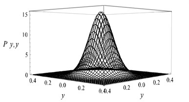
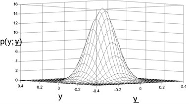
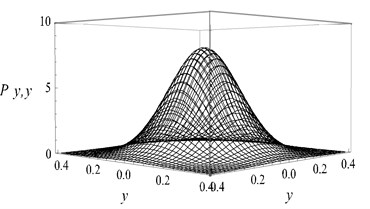
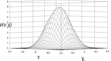
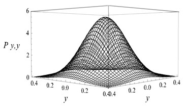
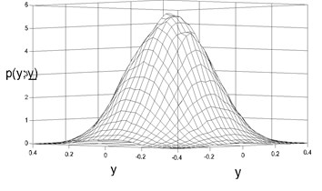
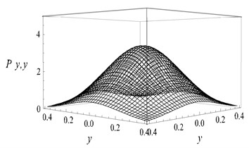
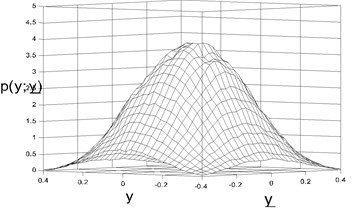
The parameters in simulation were chosen as the same as those chosen in Fig. 1. 40×40 grids were subdivided between displacement$-0.4\le y\le 0.4$and velocity $-0.4\le \dot{y}\le 0.4$. The statistics results were shown in Fig. 2. The Fig. 2(a, c, e, g) showed the analytic results by Eq. (15), while Fig. 2(b, d, f, h) showed the numerical results. It is obvious that the analytic results coincide with the digital results.

4. Reliability and the first passage failure

In engineering applications, the amplitude is usually restrained to guarantee the safety. If the amplitude exceeds a threshold value $A_c$, the cantilever could have the risk of damage. The conditional reliability function, denoted by $R\left(\left.T\right|A_0\right)$, is defined as the probability of amplitude $A$ could endure within the safe domain $\mathrm{\Omega }=[0,A_c]$ with the time increasing for $t=$ 0 to $t=T$ given an initial amplitude $A_0$ being in the safe domain $\mathrm{\Omega }$ i.e.:

The conditional transition probability density is governed by the backward Kolmogorov (BK) equation with drift coefficient $m\left(A\right)$ and diffusion coefficient $\sigma \left(A\right)$ defined by Eq. (10). It can be shown that the conditional reliability function satisfies the following BK equation:

The initial condition and the boundary conditions associated with Eq. (17) are:

Fig. 2Stationary joint PDF of displacement and velocity: a), b) D= 0.01, c), d) D= 0.02, e), f) D= 0.03, g), h) D= 0.05)

a)

b)

c)

d)

e)

f)

g)

h)

It is reasonable to assume that the first-passage occurs once $A$ exceeds certain critical value $A=A_c$ for the first time. Obviously, conditional damage probability can be defined as following:

The conditional probability density of first passage time [17, 18] can be obtained from the conditional reliability function as follows:

When the numerical simulations were carried out, 10 000 sets of noise for each noise density $D$ were imposed to the system. Each set has 2 000 numbers with a time step 0.05, which means the reliability within10 units of dimensionless time was calculated, i.e. $T=$ 10 in Eq. (16). Initial value was taken as $A_0=$ 0, and the threshold value was taken as $A_c=$ 0.2. The reliability can be seen in Fig. 3.

Both the theoretical solutions and digital simulation results were all given in Fig. 3. During the numerical simulation, 10 000 sets of noises signal were imposing into this system Eq. (4) for each noise density. Subsequently, we chose a time gap as 0.25, which mean statistic would be done at dimensionless time nodes 0.25, 0.50, 0.75 $\cdots$ 10. At each time node $n$×0.25, $n=$1, 2, 3,…, 40, we counted the numbers of the noise input sets $N$ could guarantee the maximum amplitude less than $A_c=$ 0.2 within the time span $[0,n\times 0.25]$. Then we calculated the percentage of the reliability $R\left(t\right)$ by $N/10000$ at each time node. The separated dots in Fig. 3 are the statistic results. The precision of the BK function predicting the reliability of the actuator is good enough in view of the fact that the digital dots obtained by simulation directly of Eq. (4) are so close to the solid lines solved form Eq. (17) by finite difference method. The errors exist because the diffusion coefficient and draft coefficient in Eq. (17) are just approximations solved by stochastic averaging. However, when the noise density is weaker the reliability decreases slower and the prediction accuracy is better. And the lager the noise density becomes, the faster the reliability decreases and the more visible the error becomes.

Similar to the numerical procedure in Fig. 3, the time gap was chosen as 0.25, we counted the times of the responses exceed $A_c=$ 0.2 for the first time for each set of noise inputs. We can understand the Fig. 4 like this: for example, the peak value of the curve noted by $D=$ 0.05 has a horizon coordinate $t=$ 0.7, which means under the noise density $D=$ 0.05 the response amplitude will most probably exceed $A_c=$ 0.2 at time 0.7. In other words, the system will not be guaranteed to be safe after 0.7 dimensionless time.

Fig. 3Reliability function of the amplitude (solid lines: theoretical results; dots: numerical simulation)

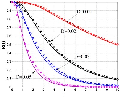
Fig. 4probability density of the first passage failure time (solid lines: theoretical results; dots: numerical simulation)

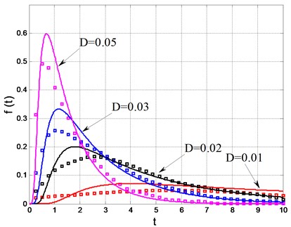
The probability of first passage failure time given by Eq. (22) differs from the digital results slightly at the peak position. We see the theoretical peak value is higher than the digital value. However, the time coordinates in accordance with the peaks are almost the same. For application, people only need to know when the amplitude will most likely to exceed the threshold value $A_c$.

5. Prediction-correction method

When the noise density is large, as seen in Fig. 1, the $A$ coordinate associated with climax of PDF curve noted by $D=$ 0.05 reached 0.2, which means the tip end of the cantilever has an amplitude as large as 20 % of the beam length. In this circumstance, ${\alpha }_2{y}^2$ cannot be assumed as far less than 1. Thus, the approximation $1/1+{\alpha }_2{y}^2\doteq 1-{\alpha }_2{y}^2$ should be modified. ${\alpha }_2{y}^2$ can be assumed that it nearly equals to one undetermined constant k which is to be predicted by formal standard stochastic averaging PDF Eq. (14). The new transformation can be obtained as:

Substituting Eq. (23) into the linear stiffness term ${\omega }_0^{2}y/1+{\alpha }_2{y}^2$ in Eq. (4) and keeping the other terms unchanged to minimize the truncation error, Eq. (4) can be rewritten as:

Applying the stochastic averaging on Eq. (24) yields the draft coefficient $m\left(A\right)$ and the diffusion coefficient ${\sigma }^2\left(A\right)$:

where:

Substituting Eq. (25) and Eq. (26) into Eq. (13) yields the modified stationary PDF of amplitude:

where:

In Fig. 1, when $D=$ 0.05, it is obvious that the amplitude $A$ in accordance with PDF peak value is about 0.21, and considering ${\alpha }_2=$ 0.4569, ${\alpha }_2{y}^2$ is nearly equals to 0.2, then it is reasonable to choose $k=$ 0.2 in Eq. (27). This procedure is the so called prediction correction method

Then, considering the conservative part of Eq. (4) kept to third-order nonlinearity is ${\omega }_0^{2}y+({\alpha }_1-{\omega }_0^2{\alpha }_2)y^3$, the influence of the three-order nonlinearity term to the response frequency cannot be neglected. The amplitude expression in numerical simulation $A=\sqrt{y^2+{\dot{y}}^2/{\omega }_0^2}$ is unsuitable anymore. We should find a more appropriate expression of amplitude in view of energy point.

The Hamilton of the system is:

Substituting $y=A\mathrm{c}\mathrm{o}\mathrm{s}\theta$ and $\dot{y}=-A\nu \mathrm{s}\mathrm{i}\mathrm{n}\theta$ into Eq. (28), where $\nu$ is a varied and undetermined frequency, and letting $\theta =$ 0, finally we obtain:

It was solved as:

Using Eq. (28) and Eq. (30) instead of $A=\sqrt{y^2+{\dot{y}}^2/{\omega }_0^2}$ in numerical simulation, and choosing $k=$ 0.2 and $D=$ 0.05, the corrected stationary PDF can be illustrated in Fig. 5.

Fig. 5Stationary PDF with D= 0.05 (solid lines: modified theoretical results; dashed lines: original results; dots: numerical simulation)

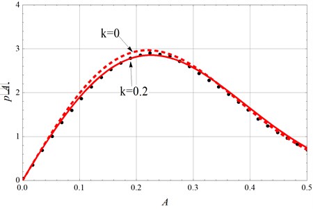
The solid line in Fig. 5 is the result of the prediction-correction method with $k=$ 0.2, the dashed line presents $k=$ 0, and the dots present the numerical results using Eq. (28) and Eq. (30). It is clear that using the prediction-correction method and considering the affect of the nonlinearity to the frequency sufficiently can improve the performance of predicting the system’s response.

6. Conclusions

In this paper, an in-extendable cantilever model subject to basal transversely Gaussian noise excitation was studied. The inertia nonlinearity and geometrical nonlinearity is taken into account sufficiently, which is the highlight of this paper. The conclusions are summarized as follows:

1) The standard stochastic averaging method is effective in predicting responses of the cantilever when the noise density is not too large i.e. the maximum response amplitude of the free end is restrained to less than 15 % of the cantilever length. The theoretical stationary PDF of amplitude, joint PDF of displacement and velocity, the reliability function and the probability density of first passage failure time are all agree with the numerical simulations. The noise density in accordance with amplitude of the tip end less than 15 % is suitable for the standard stochastic averaging method.

2) Nonlinear stiffness can influence the response frequency with considerable noise density, which increases the error of predicting PDF. Especially, when the maximum amplitude exceeded 20 % of the cantilever length the error would become significant. Also, the approximation of the inertia nonlinearity term will cause truncation error.

3) Applying prediction-correction method, modifying the approximation of the inertia nonlinearity term, and using the amplitude expression in view of energy point will help in improving the accuracy of theoretical prediction.