Cognitive design of products for engineering and vibromechanics by criterion of minimization labor input of their manufacturing

1. Introduction

The ability to quickly assess the cost of the designed products at an early stage will allow to optimize material requirements needed for the production of products, and will even allow to optimize even before creation of the first pilot products in the available ranges a product design.

The problem of estimation of the cost of production of separate parts, where it is not a precise calculation of material consumption norms and standards of operational time, namely the evaluation of the first approximation.

The basis of the algorithm for determining the labor input are user-configured according to the parameters of its real production [3]. This lays the material parameters, the actual processing of the individual elements of geometry and cost parameters of auxiliary operations. All cost characteristics tied to specific units of available equipment and tools and specific assortments. Furthermore, we define the auxiliary and preparatory operations. Finally, here adjusted cost of operations not related to the transformation of the mold material, such as coloration, control, heat treatment, etc. Any cost parameters can be used for single parts, manufactured at the same time the party or to the entire quantity of manufactured parts, and they can be assigned automatically or interactively. Cost of items will be calculated according to the template settings and according to the actual part geometry. Will also be added the costs of setting up the equipment and any additional operations and costs referred to as a template are required for use.

So, the solution offers a wide range of tools for the analysis of future product costs. And they can be used together and separately. For example, in the early stages of designing the designer can minimize the expected cost of the product by changing the design solutions, its head by a reporting engine will evaluate the range of materials and assortments and will issue guidelines to reduce it, and the technology and setters will calculate the final demand for materials and labor.

2. The calculation of labor costs with the use of an information system based on fuzzy decision trees

2.2. Pre-processing of the input data

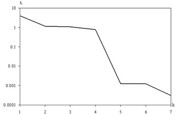
Presented in Table 1 data is analyzed to identify correlations between variables by principal component. The user receives a graph on the screen of the spectrum of the eigenvalues, such as Fig. 1.

The Fig. 1 shows that significant are the first four ingredients. Therefore, the user can reduce the number of input variables to 4.

Fig. 1The spectrum of eigenvalues

2.3. Construction of tree and base of rule

Using the above algorithm builds the appropriate decision tree. For the number of classes corresponding to the output variable on a sample of 84 items (70 %-th of sample) constructed a decision tree for all input properties (Fig. 2).

The variables $X\left[i\right]$ correspond to the properties of $D$, $d$, $H$, $h$, $Pz$, $Pm$, $Pc$.

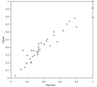
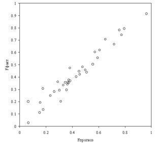
These rules can be entered in the knowledge base and used for forecasting labor products were not part of the training set. Comparison of predicted and actual work is represented in Fig. 3. When comparing the value of labor costs given in the range [0, 1].

Fig. 2The decision tree corresponding to the full set of Table 4.1 properties

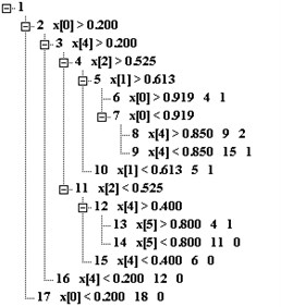
Fig. 3Comparison of predicted and actual work

This tree contains 17 units and corresponds to the following set of nine rules:

0 if X[4] >= 1.80 AND X[2] >= 17.60 AND X[1] >= 27.00 AND X[0] >= 253.80 then Y = 1

1 if X[0] >= 74.80 AND X[2] >= 17.60 AND X[1] >= 27.00 AND X[0] < 253.80 AND X[4] >= 4.40 then Y = 2

2 if X[0] >= 74.80 AND X[4] >= 1.80 AND X[2] >= 17.60 AND X[1] >= 27.00 AND X[0] < 253.80 AND X[4] < 4.40 then Y = 1

3 if X[0] >= 74.80 AND X[4] >= 1.80 AND X[2] >= 17.60 AND X[1] < 27.00 then Y = 1

4 if X[0] >= 74.80 AND X[2] < 17.60 AND X[4] >= 2.60 AND X[5] >= 3.40 then Y = 1

5 if X[0] >= 74.80 AND X[2] < 17.60 AND X[4] >= 2.60 AND X[5] < 3.40 then Y = 0

6 if X[0] >= 74.80 AND X[4] >= 1.80 AND X[2] < 17.60 AND X[4] < 2.60 then Y = 0

7 if X[0] >= 74.80 AND X[4] < 1.80 then Y = 0

8 if X[0] < 74.80 then Y = 0.

The correlation coefficient between forecast and actual values was 0.75. The mean forecast error was 7.4 %.

A decision tree can be reset by the use of compression of input data by the method of principal components.

Table 2 shows the results of calculation of the eigenvalues and the corresponding eigenvectors input from the Table 1.

The first four components are formed on the basis of the following relations:

1

$y_1=0.4981D+0.4979d+0.4980H+0.4980h-0.0594Pz-0.0298Pm+0.0604Pc,$

2

$y_2=-0.0316D-0.0316d-0.0340H-0.0312h-0.5041Pz$
$+0.0403Pm+0.7612Pc,$

3

$y_3=0.0306D+0.0331d+0.024H+0.031h+0.6507Pz+0.7562Pm+0.0355Pc,$

4

$y_4=-0.013D-0.0139d-0.0069H-0.0078h+0.5648Pz-0.5146Pm+0.6447Pc,$

Table 2The results of calculations of the eigenvalues and the corresponding eigenvectors

No	1	2	3	4	5	6	7
$\lambda$	4.0208	1.1452	1.0603	0.771	0.0013	0.0012	0.0003
	0.4981	–0.0316	0.0306	–0.013	–0.1159	–0.027	0.8577
	0.4979	–0.0316	0.0331	–0.0139	–0.5346	–0.5641	–0.3818
$w$	0.498	–0.034	0.024	–0.0069	0.8199	–0.2074	–0.1871
	0.498	–0.0312	0.031	–0.0078	–0.1687	0.7987	–0.2892
	–0.0594	–0.5041	0.6507	0.5648	0.0008	–0.0017	0.0014
	–0.0298	0.403	0.7562	–0.5146	0.0084	0.0013	–0.0014
	0.0604	0.7612	0.0355	0.6447	–0.0012	–0.0028	0.0012

Fig. 4A decision tree was built on four main components

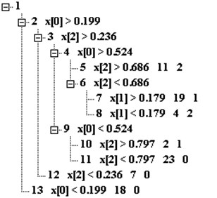
Fig. 5Comparison of predicted and actual work by using principal component analysis

Now as an input variable $X\left[i\right]$ are the components $y_1$, $y_2$, $y_3$, $y_4$. The corresponding tree shown in Fig. 4.

From a comparison of fig. 2 and 4 shows that the tree has a less complex structure and the number of sites decreased from 17 to 13. The tree corresponds to the following rules:

0 if X[0] >= –0.08 AND X[2] >= 0.79 then Y = 2

1 if X[2] >= –1.11 AND X[0] >= –0.08 AND X[2] < 0.79 AND X[1] >= –1.30 then Y = 1

2 if X[2] >= –1.11 AND X[0] >= –0.08 AND X[2] < 0.79 AND X[1] < –1.30 then Y = 2

3 if X[0] >= -2.33 AND X[0] < –0.08 AND X[2] >= 1.26 then Y= 1

4 if X[0] >= -2.33 AND X[2] >= –1.11 AND X[0] < -0.08 AND X[2] < 1.26 then Y = 0

5 if X[0] >= –2.33 AND X[2] < –1.11 then Y = 0

6 if X[0] < –2.33 then Y = 0.

The number of rules has also been reduced from 9 to 7. With a smaller number of rules has increased the quality of the forecast. Fig. 5 shows a comparison of projected and actual work.

The correlation coefficient between forecast and actual values increased to 0.833, and the mean-square prediction error decreased to 5.2 %.

As you can see, a trained information system based on using decision trees fuzzy inference copes well with the estimate of labor costs in value terms.

3. Software for the development of systems of fuzzy logic

Currently, fuzzy logic systems are widely used to control various technical systems and production process [4, 5]. In this regard, the number of software products that provide design of fuzzy systems and modeling of them, is sufficiently large. Regarding evolutionary algorithms, the software designed for their design, in wide use have. This is due to the fact that evolutionary algorithms cannot be used in general – by using configuration they require a specific situation [6].

Most software products provide the ability to design systems, fuzzy logic, based on the following stages:

1) editing of the input variables;

2) partition the domain of input variables at several intervals and each interval mapping its linguistic meaning (e.g., “low”, “medium”, “high”);

3) definition of the type of membership functions and parameters of membership functions for each linguistic variable;

4) partition of determining the output variable at several intervals, each interval mapping of linguistic meaning, definition of the type and parameters of membership functions for each output variable;

5) reference knowledge base as a production model. As productions parcels used linguistic values of the input variables are taken as prisoner’s linguistic values of the output variable;

6) defuzzification method definition output variable. Types defuzzification may vary depending on the particular software product. Basic techniques – method of the first peak, the method of the central peak, centroid method;

7) view fuzzy system in action.

Stages 2, 3 and 4 constitute the process of fuzzification (reduction to fuzziness).

A significant software product is the Matlab programming environment developed by Mathworks. Matlab is the language of mathematical data processing and provides a great number of libraries, including both purely mathematical functions and tools to design and study the properties of control systems, digital signal processing, neural networks, image processing, fuzzy logic, and even electrical and power circuits.

Matlab medium of its functionality far exceeds other packages of mathematical data processing. Tools for working with fuzzy logic in using Matlab collected in Fuzzy Logic Toolbox software package. Main features of the package: the construction of fuzzy inference systems (expert systems, regulators, approximators dependencies); Construction of adaptive fuzzy systems (hybrid neural networks); interactive dynamic simulation in Simulink package. The package allows you to work in GUI mode or in command line mode

Development of systems of fuzzy logic in the GUI mode, the program allows for Fuzzy Inference System Editor (FIS Editor) – editor-fuzzy inference system, part of the package Fuzzy Logic Toolbox Matlab programming environment. This editor allows you to carry out all stages of the design standard fuzzy systems described at the beginning of this section. In the Matlab environment supports the creation of fuzzy systems of two models: Mamdani and Sugeno.

As methods of defuzzification methods are used (Fig. 6) of the first peak (lom), the average maximum (mom), the last peak (som), the centroid (centroid), as well as any defuzzification functions, user-designed.

Easy to work with fuzzy logic systems in Matlab environment due to the presence of additional means of mass visual design, providing the modeling of fuzzy systems and facilitate the development of fuzzy systems at its various stages [1, 2].

These tools include: Membership Function Editor – editor of the membership functions, allows an fuzzification variables, choosing membership functions and their parameters in interactive mode; Rule Editor – rules editor; Rule Viewer – visualizer rules allow you to see the process of getting the result of fuzzy inference system according to various inputs; Surface Viewer – visualizer response surface; Clustering – clustering software; ANFIS Editor – editor of hybrid systems, generates and training models fuzzy Sugeno.

The essence of the editor is to generate a hybrid neural network. This neural network simulates the operation of a fuzzy logic system. In it a number of the neurons responsible for the fuzzification of the input parameters, a number of – of the rules, a number of – for the defuzzification of the output variable. From the values of the weighting factors such neural network can uniquely restore the system of fuzzy logic. These construction principles allow the use in teaching methods of fuzzy system, identical methods of training of artificial neural networks.

Fig. 6Options defuzzification in Matlab package

4. Conclusions

Use effective approach to creating an automated method of valuation, which is a generalization of the method of analogies. This valuation method is based on the construction of fuzzy decision trees, establishing depending complexity of labor in terms of value, and the parameters of the trees turn different for each of the object and take into account factors that are not related to the complexity of products, but the impact on labor intensity: the equipment used, qualification of workers, conditions labor and other indicators of organizational and technical level of production. It was found that this method provides high accuracy and adaptability.

Created labor regulation system, built on the theory of fuzzy decision trees, in which the generation of the rules and the selection of the parameters of membership functions are carried out in dynamic process of learning from the available data. Since the fuzzy learning system makes use of genetic optimization algorithms, such a system is a genetic fuzzy system or adaptive fuzzy inference system with genetic algorithm training.