The use of decision trees for applying the method of analogy with the cognitive design of complex dynamical systems

1. Introduction

Currently we considered the various valuation methods of machining settlement-analytical; research-analytical; research-statistical; total; method of analogy; direct observation; enlarged; micronutrients method and other. These methods largely overlap with each other [1, 3, 4].

In the method of analogy rules established by comparing the complexity and scope of the job on the rated work with those doing the job on the basis of the experience quantity surveyor (technologist).

The method of analogies is actually an expert method. Modern intelligent methods to extract knowledge from data allow the use of the available material for evaluation of the complexity of parts of different class, identify any patterns in the data and, thus, replace expert - technologist (quantity surveyor). In the analysis of pre-production, it is also advisable to go by the time required to manufacture the product to the price tag.

Method of analogy is based on solving the problems of classification trees using algorithms solutions [2]. These algorithms are used to solve classification problems. In the search for the classifying rule is carried out through all of the independent variables and the most representative sought a rule at this stage. These are divided into two groups according to the value of this predicate. Thereafter, the process is repeated for each of these groups as long as the resulting subgroups contain the representatives of classes and include a sufficiently large number of points to be significantly broken down into smaller subgroups. As a result, the final classifying rule constructed by this process can be represented as a binary tree.

2. Classification method based on a decision tree

Let the target variable corresponds to certain classes, which are divided a plurality of data. Required to find a classifying rule that allows to break a lot of data on these classes. In the search for the classifying rule is carried out through all of the independent variables and the most representative sought a rule at this stage. Predicates of the type $x\le w$, $x>w$ are used in the conventional decision tree. These are divided into two groups according to the value of this predicate. Thereafter, the process is repeated for each of these groups as long as the resulting subgroups contain the representatives of classes and include a sufficiently large number of points to be significantly broken down into smaller subgroups. As a result, the final classifying generally constructed by this process can be represented as a binary tree. Each node of the tree corresponds to a subset of the data and has found the classifying rule for that subset.

Convenient to analyze decision trees feature is the presentation of data in a hierarchical structure. Compact tree takes a picture of the influence of various factors, independent variables.

Classification method based on a decision tree has as advantages the following properties: a fast learning process; generation rules in areas where the expert is difficult to formalize their knowledge; removing rules in natural language; intuitive classification model; sufficiently high prediction accuracy, comparable with other methods; the construction of non-parametric models.

These positive properties approximate the methodology of decision trees to systems based on fuzzy logic, winning them in the speed of the learning process [5].

Decision trees – one of the methods of knowledge extraction from data [6]. We introduce the basic concepts of the theory of decision trees: object - example, pattern observation point in space attributes; attribute – a sign, the independent variable, the property; class label – the dependent variable, the target variable, a sign that defines the object’s class; node – internal tree node, the node checks; list – the final node of the tree, the decision node; check – a condition in the node.

Decision trees – this is a way of representing rules in a hierarchical, coherent structure, where each object corresponds to a single node, which gives a solution. Under the rule refers to a logical structure, presented in the form of: if A then B ($A\to B)$.

Let there be given a training set $X$, containing objects, each of which is characterized by $m$ attributes and one of them points to the object belongs to a particular class. This set is denoted by $X=\left\{{\mathbf{x}}^j,C_k^j\right\}$, $j=\overline{1,N}$, $k=\overline{1,K}$, where each element of this set is described by the attributes $\mathbf{x}=\left(x_i\right)$, $i=\overline{1,m-1}$ and belongs to one of the classes $C_k$. The number of examples in the set is equal to the power of this set is $\left|X\right|$. Through the $\left\{C_k\right\}$ denotes the set of classes.

Each set $X$ at any stage of decomposition is as follows:

– The set of $X$ contains a number of objects belonging to the same class $C_k$. In this case the set $X$ is a sheet defining the class $C_k$.

– The set of $X$ does not contain any object ($X=\varnothing$). In this situation it is necessary to return to a previous decomposition stage.

– The set $X$ contains objects belonging to different classes. This set is suitable for splitting into several subsets. To do this, select one of the variables in accordance with the rules $x\le w$, $x>w$ the set $X$ is divided into two subsets. This recursive process continues as long as a finite set will consist of the examples pertaining to the same class.

This procedure is the basis of many algorithms of decision trees (separation and capture method). Construction of the tree decision takes place from top to bottom. First, it creates the root of the tree, then the descendants of the root, etc.

Since all objects have been pre-assigned to certain classes, such a process of building a decision tree called learning with a teacher.

In the construction of decision trees is necessary to solve the following tasks: Select the attribute criteria on which will partition; stop learning; pruning branches.

3. Choosing the partitioning criteria

To build of the tree on each internal node is necessary to find a condition that would divides the set associated with the node in the subset. For such a test $x\le w$, $x>w$ is one of the attributes should be selected. The chosen attribute must partition the set so that the result obtained in the subset composed of objects belonging to the same class, or were as close as possible to it, i.e., the number of objects from other classes in each of these sets is as small as possible.

One way to select the most appropriate attribute to the use of information-theoretic criteria.

Task is to build a hierarchical classification model as a tree from a set of objects $X=\left\{{\mathbf{x}}^j,C_k^j\right\}$, $j=\overline{1,N}$, $k=\overline{1,K}$. In the first step, there is only the root and the initial set associated with the root.

After checking, resulting in decomposition results in two (the number of terms ($x\le w$, $x>w$)) subsets and, accordingly, are of two children of the root, each of which is assigned a subset of its obtained by partitioning the set of $X=\left\{{\mathbf{x}}^j,C_k^j\right\}$, $j=\overline{1,N}$, $k=\overline{1,K}$. This procedure is then applied recursively to all subsets (the descendants of the root), etc. Any of the attributes you can use an unlimited number of times in the construction of the tree.

We define as a test $t$ any variable that takes the value of $x_i\gtrless \left(w_{ij}\right)$, $i=\overline{1,m-1}$, $j=\overline{1,n}$. Then partition $X$ verification $t$ gives the corresponding subset of $X_{ij}$, $i=\overline{1,m-1}$, $j=\overline{1,n}$. The selection criterion is determined by the information about how the classes are distributed in a variety of $X$ and its subsets, resulting in the division on the $t$.

Let $P_{liq}^k$, $k=\overline{1,K}$$i=\overline{1,m-1}$, $q=\overline{1,n}$, $l=\mathrm{1,2}$ – the likelihood of membership in the class $k$ for the attribute $i$ and $q$threshold value $x_i\gtrless \left(w_{ij}\right)$, $i=\overline{1,m-1}$, $j=\overline{1,n}$, and $P_l^k$ – the probability of falling into the $k$ class. As a measure of the expectation of the information necessary to determine the class of the object from a plurality of $X$, Shannon entropy is considered:

The amount of entropy characterizes the degree of fuzziness of system data.

Partition of the set $X$ verification $t$ corresponds to the entropy $H_{iq}=-\sum {\sum }_{k=1}^K{P}_{liq}^k{\log }_2{P}_{liq}^k$.

The selection criterion is the expression corresponding to the maximum data ordering for classes $H_{iq}\to \text{min}$.

The minimum value of entropy $H_{iq}$ corresponds to the maximum probability of occurrence of one of the classes. The selected variable number $x_i$ and the threshold value $w_{iq}$, minimizing $H_{iq}$, $\left(i,w_{iq}\right)=\text{ArgMin}{H}_{iq}$ is used to check the value of the variable $x_i$ on condition $x_i\gtrless \left(w_{iq}\right)$ and the further movement of the tree is made depending on the result.

This algorithm is applied to the subsets obtained and allows the process to continue recursively constructing the tree up until the node will not examples of one class. If in the process of the algorithm obtained assembly associated with an empty set (i.e., no example was given in the node), then it is marked as a sheet and as solutions of the sheet is selected most common immediate ancestor class from this sheet.

The threshold values for the variable $x_i^s$, $i=\overline{1,m-1}$, $s=\overline{1,N_l}$ by the expression $w_{ij}=x_i^{\text{min}}+\left(x_i^{\text{m}\text{ax}}-x_i^{\text{min}}\right)\frac{j}{M_i}$$i=\overline{1,m}$, $j=\overline{1,M_i-1}$, where $x_i^{\text{m}\text{ax}}$, $x_i^{\text{min}}$ – the maximum and minimum values of the variable $x_i^s$, $i=\overline{1,m-1}$, $s=\overline{1,N_l}$; $N_l$ – the number of elements of a subset of breaking.

As already noted, all numerical tests are binary, i.e., share tree node into two branches.

Rule stop of partitioning node based on the fact that the partition should not be trivial, i.e., the resultant components must be at least a predetermined number of examples of $N_l^{\text{min}}$.

The degree of fuzziness of the data system may be determined by a probabilistic process (1), or by possibilistic.

Instead of probability to define a possibility of accessory to the class $k$$F_{liq}^k$, $k=\overline{1,K}$, $i=\overline{1,m}$, $q=\overline{1,n}$, $l=\mathrm{1,2}$ – by attribute $i$ and $q$ to threshold $x_i\gtrless \left(w_{ij}\right)$, $i=\overline{1,m}$, $j=\overline{1,n}$ value, and $F_l^k$ – a possibility of hit in a class $k$. The measure of an opportunity is defined by expression of $F=\frac{f_k}{\underset{k}{\max }{f}_k}$.

The Possibility measure fuzziness data system is determined by the formulas:

or:

Function $c\left(F,L\right)=\left\{F_k\ge L\right\}$ is called the function level $L$. Possibilistic approach for determining the partitioning criterion is preferable in the case of a limited number of points in the training set.

4. Test method

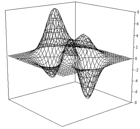
Consider the procedure of constructing of a tree of solutions on the example of the test function. This feature is rather complicated topology and described by the expression:

The form of this function for the $x_i\in \left[-\mathrm{3,3}\right]$, $i=\mathrm{1,2}$ is shown in Fig. 1.

Fig. 1Graph a test function

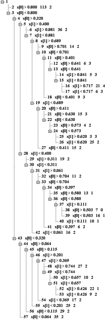
Data for the learning sample in an amount of 1089 points ${\left(x_1,x_2,\psi \right)}^j$, $j=\overline{\mathrm{1,1089}}$ generated randomly. For the training sample is divided into two roughly equal parts - training (544 points) and test (545 points). Function values $\psi$ evenly divided into $K=5$ part and form a $k=\mathrm{0,1},2$ classes. Built tree contains 57 units and is represented in Fig. 2.

After the node number should be a condition of the form $x_i\gtrless \left(w_{ij}\right)$, for it is the number of objects in a selected set. The latter figure refers to the leaves and meets the class number, which is related object satisfying these conditions. The values $x_i$, $w_{ij}$ are given in a dimensionless form.

Fig. 2View constructed tree

The resulting decision tree correspond to the following 29 rules of classification:

0 if X[0] >= 1.79 then Y= 2

1 if X[0] < 1.79 AND X[0] >= -1.08 AND X[1] >= 2.28 then Y= 2

2 if X[0] < 1.79 AND X[1] < 2.28 AND X[1] >= 1.13 AND X[0] >= 1.20 then Y= 2

3 if X[1] < 2.28 AND X[1] >= 1.13 AND X[0] < 1.20 AND X[0] >= 0.84 then Y= 3

4 if X[1] < 2.28 AND X[0] >= -0.60 AND X[0] < 0.84 AND X[1] >= 2.04 then Y= 3

5 if X[0] >= -0.60 AND X[0] < 0.84 AND X[1] < 2.04 AND X[1] >= 1.30 then Y= 4

6 if X[1] >= 1.13 AND X[0] >= -0.60 AND X[0] < 0.84 AND X[1] < 1.30 then Y= 3

7 if X[0] >= -1.08 AND X[1] < 2.28 AND X[1] >= 1.13 AND X[0] < -0.60 then Y= 3

8 if X[0] < 1.79 AND X[1] >= -0.60 AND X[1] < 1.13 AND X[0] >= 0.78 then Y= 3

9 if X[1] >= -0.60 AND X[1] < 1.13 AND X[0] < 0.78 AND X[0] >= 0.43 then Y= 2

10 if X[1] < 1.13 AND X[0] >= -0.54 AND X[0] < 0.43 AND X[1] >= 0.72 then Y= 3

11 if X[1] >= -0.60 AND X[0] >= -0.54 AND X[0] < 0.43 AND X[1] < 0.72 then Y= 2

12 if X[0] >= -1.08 AND X[1] >= -0.60 AND X[1] < 1.13 AND X[0] < -0.54 then Y= 2

13 if X[0] < 1.79 AND X[0] >= -1.08 AND X[1] < -0.60 AND X[1] >= -1.13 then Y= 2

14 if X[0] < 1.79 AND X[1] < -1.13 AND X[1] >= -2.63 AND X[0] >= 1.22 then Y= 2

15 if X[1] < -1.13 AND X[1] >= -2.63 AND X[0] < 1.22 AND X[0] >= 0.47 then Y= 1

16 if X[1] < -1.13 AND X[0] < 0.47 AND X[1] >= -2.33 AND X[0] >= 0.01 then Y= 0

17 if X[1] < -1.13 AND X[0] >= -0.62 AND X[1] >= -2.33 AND X[0] < 0.01 then Y= 1

18 if X[1] >= -2.63 AND X[0] >= -0.62 AND X[0] < 0.47 AND X[1] < -2.33 then Y= 1

19 if X[0] >= -1.08 AND X[1] < -1.13 AND X[1] >= -2.63 AND X[0] < -0.62 then Y= 2

20 if X[0] < 1.79 AND X[0] >= -1.08 AND X[1] < -2.63 then Y= 2

21 if X[0] < -1.08 AND X[0] >= -2.31 AND X[1] >= 1.46 then Y= 2

22 if X[0] < -1.08 AND X[0] >= -2.31 AND X[1] < 1.46 AND X[1] >= 0.94 then Y= 2

23 if X[0] < -1.08 AND X[0] >= -2.31 AND X[1] < 0.94 AND X[1] >= -0.45 then Y= 1

24 if X[0] < -1.08 AND X[0] >= -2.31 AND X[1] >= -0.79 AND X[1] < -0.45 then Y= 2

25 if X[0] < -1.08 AND X[0] >= -2.31 AND X[1] >= -1.79 AND X[1] < -0.79 then Y= 2

26 if X[0] < -1.08 AND X[0] >= -2.31 AND X[1] < -1.79 then Y= 2

27 if X[0] >= -2.62 AND X[0] < -2.31 then Y= 2

28 if X[0] < -2.62 then Y= 2,

where the values of variables correspond to $x\in \left[-3,3\right]$, $i=1,2$.

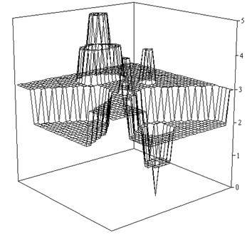
Number of correctly classified objects in the training sample is 97.4 %, and 96.9 % on the test. Fig. 3 shows the recovery of function $\psi$ in the test sample.

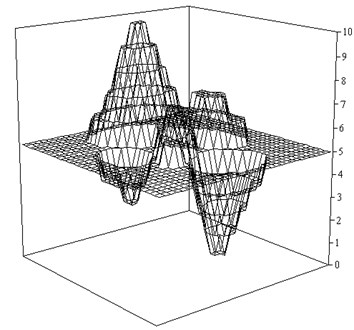
For a more detailed classification function value $\psi (x_1,x_2)$ are divided into ten classes ($K=10$). This tree contains 143 nodes and defines 64 rules. Number of correctly classified objects in the training sample is 81.6 %, 75.4 % on the test. Restore function $\psi$ in the test sample shown in Fig. 4.

Fig. 3Restore function ψ as a result of a discrete classification (K=5)

Fig. 4Restore function ψ as a result of a discrete classification (K=10)

Despite the fact that Fig. 4 can “guess” the type of a given function $\psi (x_1,x_2)$, it is clear that more appropriate methods should be used for the approximation of continuous functions.

5. Conclusion

In the article the authors presented an effective approach to the creation of the automated method of rationing production of parts and components of mechanical engineering structures, which is a generalization of the method of analogies. This valuation method is based on the construction of fuzzy decision trees, establishing depending complexity of labor in terms of value, and the parameters of the trees turn different for each of the object and take into account factors that are not related to the complexity of products, but the impact on labor intensity: the equipment used, qualification of workers, conditions labor and other indicators of organizational and technical level of production changing in dynamics. It was found that this method provides high accuracy and adaptability.