Recognition of rock–coal interface in top coal caving through tail beam vibrations by using stacked sparse autoencoders

Zhang, Guoxin; Wang, Zengcai; Zhao, Lei

doi:10.21595/jve.2016.17386

Journal of Vibroengineering

Browse Journal

Submit article

Published: 15 November 2016

Check for updates

Recognition of rock–coal interface in top coal caving through tail beam vibrations by using stacked sparse autoencoders

Guoxin Zhang¹

Zengcai Wang²

Lei Zhao³

^{1, 2, 3}School of Mechanical Engineering, Shandong University, Jinan, China

^{1, 2, 3}Key Laboratory of High Efficiency and Clean Mechanical Manufacture (Shandong University), Ministry of Education, Jinan, China

Corresponding Author:

Zengcai Wang

Cite the article Download PDF

Downloads 1843

WoS Core Citations 18

CrossRef Citations 18

Abstract

This paper provides a novel rock-coal interface recognition method based on stacked sparse autoencoders (SSAE). Given their different size and hardness, coal and rock generate different tail beam vibrations. Therefore, the rock-coal interface in top coal caving can be identified using an acceleration sensor to measure such vibrations. The end of the hydraulic support beam is an ideal location for installing the sensor, as proven by many experiments. To improve recognition accuracy, the following steps are performed. First, ensemble empirical mode decomposition method (EEMD) is used to decompose the vibration signals of the tail beam into several intrinsic mode functions to complete feature extraction. Second, the features extracted are preprocessed as the inputs of SSAE. Third, a greedy, layer-wise approach is employed to pretrain the weights of the entire deep network. Finally, fine tuning is employed to search the global optima by simultaneously altering the parameters of all layers. Test results indicate that the average recognition accuracy of coal and rock is 98.79 % under ideal caving conditions. The superiority of the proposed method is verified by comparing its performance with those of four other algorithms.

1. Introduction

Coal is a highly important energy source, contributing approximately 30 % of the world’s energy consumption and 64 % of that of China in 2015. In China, the storage capacity of thick coal seam accounts for up to 45 % of the total storage. Top coal caving mining technology is widely used to mine thick coal seam because of the approach’s advantages of high production, high efficiency, low energy consumption, low cost, and strong adaptability.

However, a large problem exists in top coal caving with regard to heavy reliance on manual eyeballing for identifying the rock–coal interface. This approach easily causes owing and over caving. Owing caving results in a drop in recovery rate and resource waste amount, whereas over caving leads to decline in coal quality and rise in production cost. Over caving also brings great security risk to operators because of the extremely harsh mining environment and complex process of top coal caving. Therefore, achieving automation for top coal caving mining is an important goal. Such automation requires highly accurate and rapid recognition of coal and rocks.

In the past decades, researchers have proposed many methods for recognizing coal and rock. The most famous methods include γ-ray detection [1-3], radar detection [4, 5], cutting force response [6, 7], infrared detection [8], and image detection [9]. These methods have acquired some valuable achievements and have been applied in several fields. However, such techniques present with disadvantages. Artificial $γ$ rays are harmful to human beings, and the cost of natural $γ$ rays is also relatively high. Meanwhile, radar detection faces the problem of considerable contradiction between measuring range and precision. Meanwhile, cutting force response method is unsuitable for the top coal caving mining environment, whereas infrared detection method is insufficiently mature. In addition, the recognition accuracy rate of the above-mentioned methods is highly sensitive to the coal mine environment.

A method based on vibration signal analysis has been investigated by an increasing number of researchers [10-13] in recent years and used in many practical applications. In [10], the measuring point of arm vibration was optimized. In [11], the power spectrum of coal and rock vibration models based on a time-series analysis was employed to identify coal and rock. In [12], the shear cutting state was diagnosed by an acceleration sensor that measures the vibration of the rock transmission part. In [13], the identification of coal and rock were depended on the vibration of the rear scraper conveyor and the hydraulic support tail beam in different conditions. In comprehensive coal caving mining, they hit the tail beam of the hydraulic supporter to cause the tail beam to vibrate when coal or rocks fall. Given the different size and hardness of coal and rock, the tail beam vibration produced was different. Therefore, we can identify the rock–coal interface by using acceleration sensors to measure tail beam vibration.

The essence of rock-coal interface detection is pattern recognition and classification. Numerous suitable methods for classification exist. These approaches include probabilistic neural network [12], back-propagation neural network [14], fuzzy logic [15], support vector machine (SVM) [8, 16], and naive Bayes etc. The neural network is widely used and the most well-known among the techniques. In 1958, the neural network was first proposed [17]; since then, correlative methods have been developed; these methods include convolution autoencoders neural networks (CAE), back propagation (BP), convolution neural networks (CNN), deep belief networks (DBN), and stacked sparse autoencoder (SSAE) neural networks. These techniques differ in architecture, learning approach, and training method and hence present different performances in applications. Many successful engineering examples, such as weather prediction [18], facial expression recognition [19], fault diagnosis [20] and speech recognition [21], were developed.

The SSAE neural network is a highly effective method for classification and has been widely employed for classification and pattern recognition problems [22] since its proposal. A SSAE consists of several layers of sparse autoencoders (SAEs), in which the input of the next layer is the output of the previous layer. Greedy, layer-wise, SSAEs can pretrain the weights of the entire deep networks by training each layer. Numerous optimization algorithms were proposed in the progress of optimizing the parameters of neural networks, including genetic algorithm [7, 23], conjugate gradient descent [24], BFGS [25], L-BFGS [26], and gradient descent. In this paper, gradient descent was selected because of its simplicity and practicality.

Feature extraction is an important aspect because the vibration signal of the tail beam is non-linear and non-stationary. Some typical methods, such as wavelet transform (WT) [27], empirical mode decomposition (EMD) [28], and the Fourier transform (FT) [29] are applicable. In this paper, we selected ensemble EMD (EEMD), which was proposed in 2004 [30]. Successfully solved mode mixing, EEMD has been widely used in many industries, such as vibration analysis [31] and signal denoising [32].

The proposed method mainly included three parts. The first part is involved signal acquisition by using 4508 type acceleration sensor and 3560 B data acquisition front end to acquire the tail beam vibration signals produced by the rock and coal. The second part comprised feature extraction. EEMD algorithm was used to decompose the signals into intrinsic mode functions (IMFs) and the relatively effective components were singled out. The third part consisted of the recognition of the rock–coal interface using a SSAE neural network based on batch gradient descent algorithm to recognize of coal and rock. To establish the SSAE model, we conducted many experiments to obtain the optimal parameters for SSAE.

2. Materials and methods

For many years, neural networks have been widely used in classification and obtained favorable results. This paper proposed a novel network model named SSAE to recognize the rock-coal interface in top coal caving. The SSAE first initializes parameters and then uses feed-forward and back-propagation by batch gradient descent algorithm to seek the minimum of cost function for obtaining the global optical parameters. The progression is called pretraining, which involves unsupervised learning. Afterward, fine-tuning is employed to obtain better results. In fact, the SSAE holds a powerful expression and enjoys all the benefits of deep networks. Furthermore, the model can achieve hierarchical grouping or part-whole decomposition of the input. For example, if the input is a face image, the first layer may learn how to identify the boundaries, the second layer may learn how to combine these boundaries, and the higher layer may learn how to combine facial organs [19].

2.1. SSAE

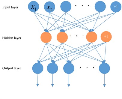
A SAE neural network is an unsupervised learning algorithm that does not require labeled training examples unlike other neural networks. Applying back propagation sets the target values to be equal to the inputs. The schematic of a SAE with $n$ inputs and $m$ units in the hidden layer is shown in Fig. 1.

Fig. 1Schematic of a SAE

In an autoencoder, the overall cost function is as follows:

1

J (W, b) = [\frac{1}{m} \sum_{i = 1}^{m} (\frac{1}{2} {‖h_{W, b} (x^{(i)}) - y^{(i)}‖}^{2})] + \frac{λ}{2} \sum_{l = 1}^{n_{l} - 1} \sum_{i = 1}^{s_{l}} \sum_{j = 1}^{s_{l} + 1} {(W_{j i}^{(l)})}^{2},

where $x^{(i)}$ is the raw input, $m$ is the number of inputs, $y^{(i)}$ is the raw output, $h_{W, b} (x^{(i)})$ is the output of activation function, $λ$ is the relative importance of the second term.

In a SAE, we can discover some correlations of input features by placing constraints on the network. Sparsity $ρ$ is imposed to constrain the hidden units as follows:

2

{\hat{ρ}}_{j} = \frac{1}{m} \sum_{i = 1}^{m} [a_{j}^{2} (x^{(i)})],

where $α_{j}^{2}$ denotes the activation of hidden unit $j$ in the SAE when the network is given a specific $x^{(i)}$ . The parameter is the average activation of hidden unit $j$ . Moreover, we make the two parameters equal as follows:

3

{\hat{ρ}}_{j} = ρ .

Typically, this parameter holds a very small value, usually 0.05. Thus, we need the activation of the hidden unit to be close to 0. We add a penalty term to penalize the situation of ${\hat{ρ}}_{j}$ deviating significantly from to optimize the objective. The penalty term is as follows:

4

\sum_{j = 1}^{s_{2}} K L (ρ | | {\hat{ρ}}_{j}) .

Then, the overall cost function is:

5

J_{s p a r s e} (W, b) = J (W, b) + β \sum_{j = 1}^{s_{2}} K L (ρ | |{\hat{ρ}}_{j}) .

The detailed establishment of SSAE, pretraining, and fine-tuning can be carried out in the following steps (Fig. 2):

Step (1): A SAE is trained on the raw input $x^{(k)}$ . for learning of primary features $h^{(1) (k)}$ . The structure of the first SAE is $[n, s_{2}, n]$ , corresponding to $n$ inputs, $s_{2}$ units in hidden layers, and $n$ outputs.

Step (2): This trained SAE is then adopted to obtain the primary feature activations $h^{(1) (k)}$ for each input $x^{(k)}$ .

Fig. 2Establishment of SSAE

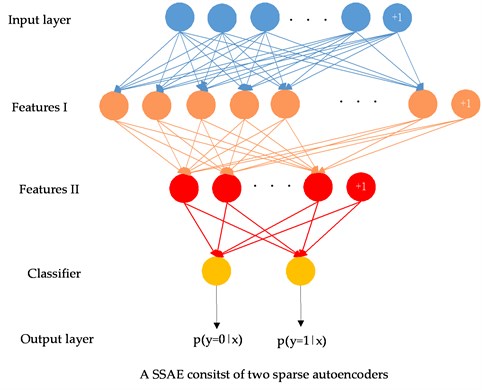
Step (3): $h^{(1) (k)}$ is then used as the “raw input” to the second SAE for learning the secondary features $h^{(2) (k)}$ . The second SAE structure is described by $[s_{2}, s_{3}, s_{2}]$ , corresponding to $s_{2}$ inputs, $s_{3}$ units in hidden layer, and $s_{2}$ outputs.

Step (4): To obtain the secondary feature activations $h^{(2) (k)}$ , each $h^{(1) (k)}$ is fed into the second SAE.

Step (5): Treat the secondary features as “raw inputs” of a sigmoid classifier to map digit labels.

Step (6): Combine the three layers and a classifier layer to form the SSAE model.

Step (7): Back-propagation is conducted to improve the results by adjusting the parameters of all layers simultaneously in a process called fine-tuning.

Step (8): Step (7) is performed repeatedly until the set training times are achieved.

2.2. Batch gradient descent

Batch gradient descent is an efficient algorithm for searching the optimal solution. One iteration of batch gradient descent is as follows:

Step 1: The following assumptions are set: $Δ W^{(l)} : = 0$ , $Δ b^{(l)} : = 0$ for all $l$ .

where $Δ W^{(l)}$ is a matrix with the same dimension as $W^{(l)}$ and $Δ b^{(l)}$ is a vector with the same dimension as $b^{(l)}$ .

Step 2: For $i = 1 : m,$ back-propagation is used to compute $\nabla_{W^{(l)}} J (W, b; x, y)$ and $\nabla_{b^{(l)}} J (W, b; x, y)$ . The following expressions are set:

6

Δ W^{(l)} : = Δ W^{(l)} + \nabla_{W^{(l)}} J (W, b; x, y),

Δ b^{(l)} : = Δ b^{(l)} + \nabla_{b^{(l)}} J (W, b; x, y),

where $W^{(l)}$ is the weights, and $b^{(l)}$ is the bias term.

Step 3: $W^{(l)}$ and $b^{(l)}$ are updated as below:

7

W^{(l)} = W^{(l)} - α [(\frac{1}{m} Δ W^{(l)}) + λ W^{(l)}], b^{(l)} = b^{(l)} - α [\frac{1}{m} Δ b^{(l)}],

where $λ$ is the weight decay parameter. The above-mentioned steps of batch gradient descent are repeated to reduce the cost function for training the neural network.

3. Recognition system for the rock-coal interface

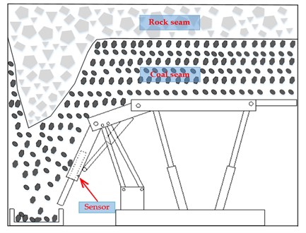
The intelligent recognition of rock-coal interface system consists of signal acquisition, feature extraction, and rock-coal interface identification and prediction (Fig. 3). Top coal caving working site is shown in Fig. 4.

Fig. 3Recognition system of the rock–coal interface in top coal caving on the basis of the proposed method

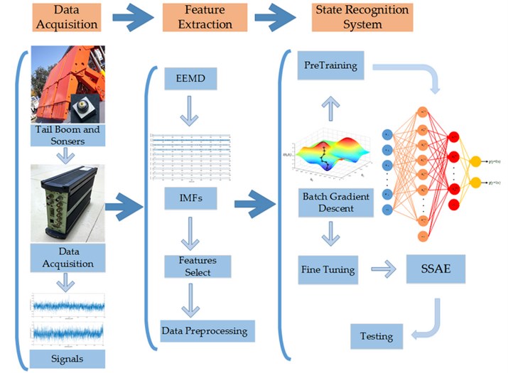
Fig. 4Top coal caving working site

3.1. Acquisition of the vibration signal of tail beam

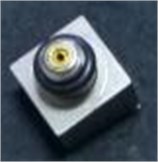
The vibration signal acquisition of a tail beam is the first step for identification of rock-coal interface. Obtaining the vibration signal by sensors is the most common method used for identification. In this study, an acceleration sensor (4508 type) was employed. Table 1 displays the acceleration sensor parameters, and Fig. 5 presents the vibration sensor.

Table 1Parameters of 4508 type acceleration sensor

Parameters	Range	Sensitivity	Frequency range	Mounted resonance frequency
Values	–71 g to 71 g	97.17 mV/g	0.5 Hz to 6000 Hz	22 kHz
Resolving power	Installation method	Sensor power supply	Temperature range	Weight
0.0002 g	Magnetic base	Constant current source power supply (2 mA to 20 mA)	–54 °C to +121 °C	4.8 g

Fig. 54508 type acceleration sensor

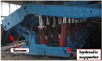
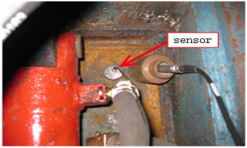
During top coal caving, coal or rock strikes the tail beam supported by a hydraulic supporter to produce vibration. Vibration waves vary because of different size and hardness of coal and rock. Detection of tail beam vibration can successful identify and differentiate coal and rock. The installation position of the sensor is important for collecting signals. After analyzing the actual working scene, we noted that the main impact locations of coal and rock are the beam and tail chute, respectively, of the hydraulic supporter. Accordingly, we set the sensors at these two places. After many experiments, we found that the sensor is easily buried by falling coal and stone when the sensor is installed in the tail chute. Moreover, the continuous spraying of water for dust-proofing may have damaged sensors during coal caving. The running conveyor chute also generated considerable interference during signal acquisition, thereby negatively affecting the next step of the analysis. Hence, the end of the hydraulic support beam is an ideal location for sensor installation. Then, we chose the tail beam back to acquire vibration signals. The final self-designed experimental system and specific installation location of the sensor are shown in Fig. 6(a) and 6(b), respectively.

The experimental data acquisition system also includes a portable vibration sound wave signal detector with a data acquisition front end, wireless routers, and software system. Vibration signals were obtained by the data acquisition front end, transmitted to the wireless broadband router by cables, and then sent to a notebook for data storage and analysis. Afterward, we exported the data from the software system. All the data were acquired in the No. 1306 working platform in the Xinglongzhuang coal mine of Yanzhou Mining Company. The working pattern involved one knife and one caving. Caving step distance determination was 0.8 m, and coal thickness was 7.34 m to 8.90 m. The frequency of sampling was set as 2560 Hz, and each pattern’s sampling time was 160 ms. A total of 4096 sampling points were obtained for each pattern, and 4000 sample points were saved for each pattern to avoid possible errors of uncertainty.

Fig. 6a) Experimental system; and b) specific installation location of the sensor

a)

b)

3.2. Feature extraction

Features must be extracted from the data exported from the pulse to enable the use of pattern recognition training and rock-coal interface prediction. Obtaining the final recognition results is hence a highly important task.

Many signal processing approaches can obtain desirable features from primary vibration signals and widely used in many industries, such as the FT [27, 28], WT [29], and EMD [30]. However, the signal was submerged in a strong background noise and non-stationary signals because of difficulty extracting useful features. For example, a signal based on the local characteristic time scales could be decomposed into several IMFs by EMD. However, it exists the problem of mode mixing. Thus, EEMD [29] was presented to solve this problem. Compared with EMD, EEMD adds a certain amount of Gaussian white noise to the original signal to solve mode mixing each time before decomposing. EEMD is highly useful for non-stationary and non-linear signals.

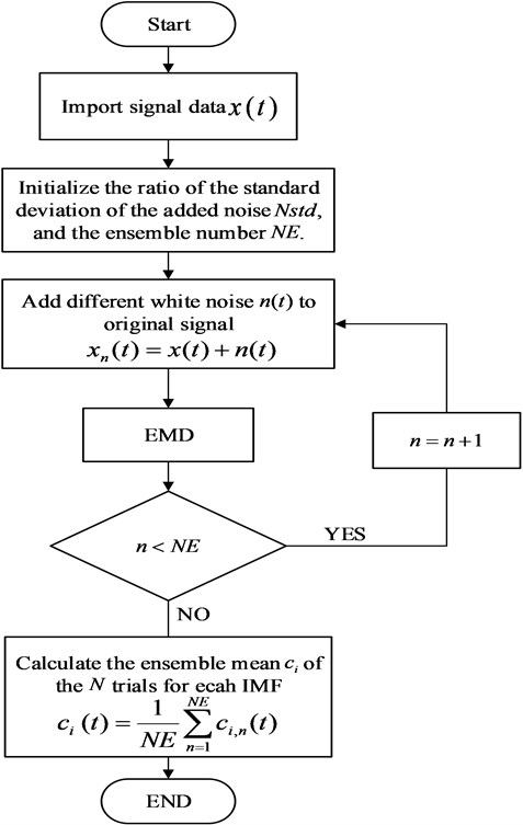
The followings are the summary of EEMD (Fig. 7):

Step 1: The standard deviation of the added noise $N s t d$ and the ensemble number $N E$ is initialized. The experiments show that the proposed model obtained better recognition when we set $N E =$ 300 and $N s t d =$ 0.2.

Step 2: Different white noises with different standard deviation are added to the original signal.

8

x_{m} (t) = x (t) + n (t),

where $x_{m} (t)$ signifies the added signal, $x (t)$ represents the original signal, and $n (t)$ denotes the nth added white noise.

Step 3: The added noise signal is decomposed by EMD into $N$ IMFs.

Step 4: If $n < N E$ , $n = n + 1$ and steps (2) and (3) are repeated; otherwise, the next step is performed.

Step 5: Each IMF is calculated by the ensemble mean $c_{i} (t)$ of the $N$ trials as follows:

9

c_{i} (t) = \frac{1}{N E} \sum_{n = 1}^{N E} c_{i, n} (t), n = 1,2, . . ., N E .

Fig. 7EEMD flowchart

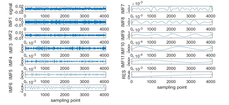
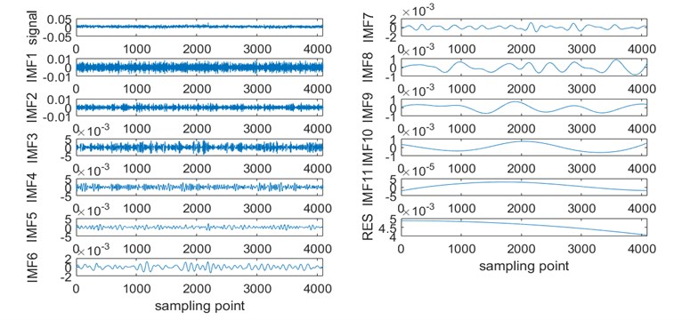
By using the EEMD algorithm, we decomposed the primary vibration signal to 11 IMFs (Fig. 8).

But the IMFs obtained by EEMD are not always the intrinsic mode functions. This is because when the EEMD decomposed the signal, the addition of white noise leads to the high frequency components maybe actually white noise, but not the intrinsic mode functions and should be deleted. Significance test and orthogonality check are conducted, and the significances shows that the first four IMFs have no significance relationship with the results. We removed the first four IMFs and the correctness of it is proved by the experiments in Section 3.3.2.

In the following data processing, these remained IMFs were used as inputs for the proposed model in the working pattern recognition. Before importing these features to the SSAE model, we first conduct preprocessing. Such step must first be accomplished because the input vectors cannot exceed the defined scope of the hidden and output layers. Through this manner, we can full apply the value of each input and render the operation more convenient and fast. In fact, the normalized method is first used to limit the input absolute value to between 0 and 1, then the standard normal state method is adopted to transform the input into a standard normal distribution.

In these studies, 4000 groups of samples were obtained for each pattern and 8000 groups in total. In the following experiments, a 10-fold cross validation method was employed, and samples were randomly divided into 10 portions. Nine portions were utilized to train the proposed model, whereas 1 portion was used for testing. Each subsample was tested once, and the average of the results of the 10 experiments was regarded as the final test result. In each experiment, 7200 samples were adopted for training, and 800 samples were used for testing.

Fig. 8Signal, decomposed components by EEMD, and trend term (RES): a) coal, b) rock

a)

b)

3.3. Construction of a SSAE model

To establish the proposed model, we carried out numerous experiments using the control variable method and determined basic parameters, such as learning rate and sparsity parameter. Parameters are obtained by comparing with different recognition accuracy rates of input features, classifiers, and structures.

3.3.1. Basic parameters

During the reduction of cost function by batch gradient descent, if the learning rate $α$ is excessively large, which results in an excessively large step size, gradient descent may overshoot the minimum and deviate increasingly further from the minimum. Setting the learning rate $α$ as exceedingly small is also unreasonable because such action can slow down the computing speed entailed to reduce the cost function. Another drawback is the potential trapping in the local optima and the potential resultant inability to reach the global optimal solution. In this proposed model, we set $α$ as equal to 1.25. By changing only one parameter and fixing the others, we can obtain the values of the other parameters, such as the number of samples in batch training $b a t c h s i z e$ , the sparsity parameter $ρ$ , and so on. In this study, we set the $b a t c h s i z e =$ 40, $ρ =$ 0.3, and the number of SAEs as 2.

3.3.2. Comparison among algorithms with different features

In this experiment, we set the first SAE structure as [ $x_{n}$ 300 $x_{n}$ ], where $x_{n}$ is the number of input features, varying from 1 to 11. The second SAE structure was [300 40 300]; the classifier was sigmoid, and the learning rate, sparsity parameter, and other parameters were set as mentioned above.

When $x_{n}$ is 1, each preprocessed IMF is separately used as the input feature of the proposed model. Table 2 shows the recognition accuracy results. It shows that the recognition accuracies of preprocessed IMF 2 and 4 are less than 50 %, played a negative role. But preprocessed IMF 11 has got a good recognition rate (78.60 %).

Table 2Recognition accuracy rates with one feature

Preprocessed IMF	1	2	3	4	5	6
Recognition accuracy	50.04 %	49.98 %	50.10 %	49.75 %	52.05 %	51.01 %
Preprocessed IMF	7	8	9	10	11
Recognition accuracy	53.25 %	54.25 %	52.75 %	57.3 0%	78.60 %

When the number of input features is set to $i$ , $i$ preprocessed IMFs chosen from the 11 preprocessed IMFs and there are $C_{11}^{i}$ combinations of preprocessed IMFs. After $\sum_{i = 1}^{11} C_{11}^{i} =$ 2047 experiments, we sorted out the maximum recognition accuracy rates of each input features number and the corresponding combinations of preprocessed IMFs (Table 3).

Table 3Recognition accuracy rates with different features

Number of input feathers	1	2	3	4	5	6
Max recognition accuracy	78.60 %	93.19 %	95.92 %	97.30 %	97.76 %	98.21 %
Combinations of preprocessed IMFs	10	10,11	8, 10, 11	1, 8, 9, 10	6, 8, 9, 10, 11	5, 7, 8, 9, 10, 11
Number of input feathers	7	8	9	10	11
Max recognition accuracy	98.96 %	98.40 %	98.55 %	98.51 %	98.20 %
Combinations of preprocessed IMFs	5, 6, 7, 8, 9, 10, 11	4, 5, 6, 7, 8, 9, 10, 11	3, 4, 5, 6, 7, 8, 9, 10, 11	1, 2, 3, 5, 6, 7, 8, 9, 10, 11	1, 2, 3, 4, 5, 6, 7, 8, 9, 10, 11

It shows that the recognition rate achieved an initial upward then downward trend. When the number of input features set to 7, corresponding to the preprocessed IMF from 5 to 11, the recognition rate reached the maximum value (98.96 %). So we removed the first four preprocessed IMFs and use the remaining 7 preprocessed IMFs as the input of the proposed model.

3.3.3. Comparison among algorithms with different hidden layer structures

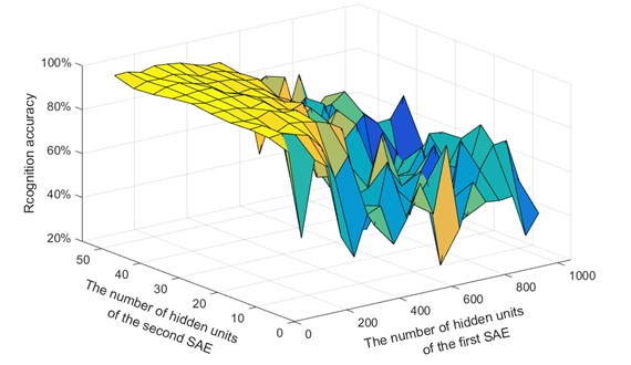
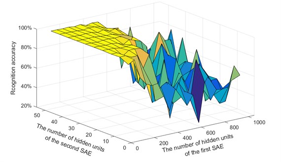
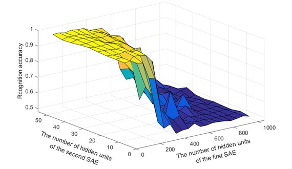
In this experiment, we set the number of first autoencoder hidden units to vary from 50 to 1000 at intervals of 50. The number of the second autoencoder hidden units varied from 5 to 50 at intervals of 5. A total of 200 kinds of different structures were assessed to find the most suitable structure for the proposed model (Fig. 9).

Fig. 9Recognition accuracy rates for different hidden layer structures: a) coal, b) rock, c) average

a)

b)

c)

Fig. 9(a), (b) and (c) refer to the accuracy rates of coal, rock, and the average of coal and rock, respectively. Fig. 9(a) shows that when the number of hidden units of the first SAE was set to 150 and the number of hidden units of the second SAE was set to 40, the accuracy of the coal reached the maximum value (98.12 %), followed by the proposed method structure of [11, 50, 30, 2] (97.95 %) and the structure of [11, 200, 50, 2] (97.85 %). Meanwhile, Fig. 9(b) reveals that the structure of [11, 200, 40, 2] enabled the recognition accuracy of rock to reach the maximum (100 %), followed by the proposed method structure of [11, 50, 30, 2] (99.98 %). Fig. 9(c) shows that the average identification of coal and rock achieved the maximum (98.96 %) when the structure was [11, 50, 30, 2].

3.3.4. Comparison among algorithms with and without pretraining

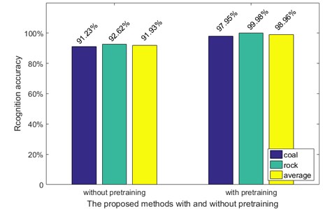
Pretraining plays an important role in the recognition of SSAE model, and the comparison of the proposed model with and without pretraining (Fig. 10).

As shown in the Fig. 10, the proposed model with pretraining works better than without pretraining, their average accuracy rates were 98.96 % and 91.93 %, respectively, and 7.03 % was improved by pretraining. This result was relatively easy to understand. Without pretraining, the network can only fine-tune the unpretrained parameters, which usually comprise some random initial points. This notion explains why the network may be confined to the local optima. With pretraining, the network could be fine-tuned on the pretrained parameters that will obtain the global optima. Thus, pretraining SSAE is a necessary step.

Fig. 10Comparison of the algorithms with and without pretraining

3.3.5. Comparison among algorithms with different classifiers

In neural networks, several classifiers are involved. In this study, three classifiers were selected. By comparing their performances, sigmoid was adopted. Their recognition accuracies are shown in Fig. 11. The sigmoid performed much better than softmax and SVM; the sigmoid obtained a 98.96 % average accuracy rate, whereas softmax only attained 50.06 % and SVM only achieved 49.01 %. Softmax and SVM both poorly recognized coal and rock. In this experiment, three models only differed in the final classifier, and the other parameters were also similar, thereby ensuring the credibility of the experiment.

3.4. Comparison and discussion

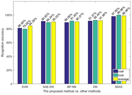
For efficient performance assessment, we compared our algorithm with other four algorithms. The four algorithms include SVM, BP neural network (BP-NN), deep network (DN), one SAE-DN. For the SAE-DN, weights were pretrained only by one SAE. For the BP-NN, weights were optimized only in the back-propagation during neural network training. To be objective and fair, the environment of simulation for the five models were rendered similar. The average results of 10 experiments are presented in Fig. 12. Obviously, SSAE operated more effectively than the other algorithms. The testing accuracy of coal, rock, and the average of the two were 97.95 %, 99.98 %, and 98.96 %, respectively. The SVM algorithm was inferior to the other methods in both the recognition of coal and rock, with accuracy rates of only 88.95 % and 79.62 %, respectively, and an average recognition accuracy of 84.29 %. The SAE-DN algorithm did not achieve a satisfactory recognition of rock (89.24 %) but performed effectively for the recognition of coal (90.83 %). The DN algorithm (91.37 %, 92.44 %, and 91.90 %) was superior to BP-NN (89.09 %, 91.45 %, and 90.47 %) but inferior to SSAE in coal and rock recognition.

Fig. 11Comparison of the algorithms with different classifiers

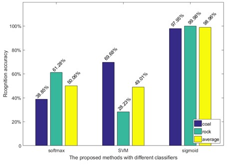
Fig. 12Results from different methods

4. Conclusions

This paper presented a novel method based on SSAE deep networks for the recognition of rock–coal interface in top coal caving. In the process, we found the most suitable installation location for the sensor. The SSAE algorithm consisted of two layers of SAE, in which the inputs of each layer were the outputs of previous layer, thereby providing the optimized weights for the deep networks. To obtain a higher diagnosis accuracy, we performed numerous experiments to obtain the global optical parameters. Furthermore, we compared the performance of our proposed approach with those of other four methods and proved the superiority of the SSAE model over the competing models.

Our study can help achieve better understanding of pattern classification or the use of SSAE deep networks. In the future works, we intend to acquire more signals of vibration because deep networks require large numbers of samples for network training. Then, we aim to use more effective feature extraction algorithms for improving the pattern recognition accuracy. We also plan to write a more efficient code that facilitates calculations and to test other efficient algorithms.

References

Bessinger S. L., Neison M. G. Remnant roof coal thickness measurement with passive gamma ray instruments in coal mine. IEEE Transactions on Industry Applications. Vol. 29, Issue 3, 1993, p. 562-565.

Publisher
Wang Z. C. Research on coal seam thickness detection by natural gamma ray in shearer horizon control. CNKI. JCCS, Vol. 27, Issue 4, 2002, p. 425-429.

Search CrossRef
Qin J. Q., Zheng J. R., Zhu X. Establishment of a theoretical model of sensor for identification of coal and rock interface by natural γ-ray and underground trials. CNKI. JCCS, Vol. 21, Issue 5, 1996, p. 513-516.

Search CrossRef
Ralston J. C., Hainsworth D. W. Application of ground penetrating radar for coal depth measurement. IEEE Conference on Acoustics, Speech, and Signal Processing, Vol. 4, 1999, p. 15-19.

Publisher
Zhang P. S., Li Y. S., Zhao Y. H. Application and analysis on structure exploration of coal seam by mine ground penetrating radar. 14th International Conference on Ground Penetrating Radar (GPR), 2012, p. 469-472.

Search CrossRef
Ren F., Liu Z. Y., Yang Z. J. Harmonic response analysis on cutting part of shearer physical simulation system paper title. IEEE 10th International Conference on Signal Processing (ICSP), 2010, p. 2509-2513.

Publisher
Tian M. Q., Xiong S. B. Previewing control system of automatic height adjustment for drum-type coal excavator based on memory cutting with identification of object model by genetic algorithm. International Conference on Machine Learning and Cybernetics, Vol. 2, 2002, p. 633-636.

Publisher
Wang Y. B. Infrared spectrum analysis of the gas in coal mine based on SVM. IEEE International Conference on Intelligent Computing and Intelligent Systems, Vol. 2, 2009, p. 608-611.

Publisher
Liu F. Q., Qian J. S., Wang X. H. Automatic separation of waste rock in coal mine based on image procession and recognition. CNKI, JCCS, Vol. 25, Issue 5, 2000, p. 534-537.

Search CrossRef
Fang R., Zheng Y. L., Zhao J. Y. Dynamics analysis for cutting part of shearer physical simulation system. IEEE International Conference on Information and Automation (ICIA), 2010, p. 260-264.

Search CrossRef
Wang B. P., Wang Z. C., Zhu S. L. Coal-rock interface recognition based on time series analysis. International Conference on Computer Application and System Modeling (ICCASM), Vol. 8, 2010, p. 356-359.

Search CrossRef
Si L., Wang Z. B., Liu X. H. Cutting state diagnosis for shearer through the vibration of rocker transmission part with an improved probabilistic neural network. Sensors, Vol. 16, 2016, p. 4-479.

Publisher
Zhu S. G., Xue G. H., Zhao X. Y. Vibration signal time-domain characteristic extraction for coal and rock recognition at the fully mechanized top-coal caving face. ICMECT, Shanghai, China, 2014, p. 2862-2865.

Publisher
Fang H. Q., He L. Human activity recognition based on feature selection in smart home using back-propagation algorithm. ISA Transactions, Vol. 53, Issue 5, 2014, p. 1629-1638.

Publisher
Winston D. P., Saravanan M. Single-parameter fault identification technique for DC motor 514 through wavelet analysis and fuzzy logic. Journal of Electrical Engineering and Technology, Vol. 8, 2013, p. 1049-1055.

Publisher
Lee Y. J., Mangasarian O. L. SSVM: a smooth support vector machine for classification. Computational Optimization and Applications, Vol. 20, 2001, p. 5-22.

Publisher
Rosenblatt F. The perceptron: a probabilistic model for information storage and organization in the brain. Psychological Review, Vol. 65, Issue 6, 1958, p. 386-408.

Publisher
Taylor J. W., Buizza R. Neural network load forecasting with weather ensemble predictions. IEEE Transactions on Power Systems, Vol. 22, Issue 7, 2002, p. 626-632.

Publisher
Wang L. K. Recognition of human activities using continuous autoencoders with wearable. Sensors Vol. 16, Issue 2, 2016, p. 189.

Publisher
Dhumale R. B., Lokhande S. D. Neural Network Fault Diagnosis of Voltage Source Inverter under variable load conditions at different frequencies. Measurement, Vol. 91, 2016, p. 565-575.

Publisher
Gandhiraj R., Sathidevi P. S. Auditory-based wavelet packet filterbank for speech recognition using neural network. International Conference on Advanced Computing and Communications, 2007, p. 663-673.

Publisher
Liu Y. N., Feng X. Q., Zhou Z. G. Multimodal video classification with stacked contractive autoencoders. Signal Processing, Vol. 120, 2016, p. 761-766.

Publisher
Kyriaki G., Helen D. K. A simulation study of multi-criteria scheduling in grid based on genetic algorithms. IEEE International Symposium on Parallel and Distributed Processing with Applications, 2012, p. 317-324.

Search CrossRef
Specht D. F., Romsdahl H. Experience with adaptive probabilistic neural networks and adaptive general regression neural networks. IEEE International Conference on Neural Networks, IEEE World Congress on Computational Intelligence, Vol. 2, 1994, p. 1203-1208.

Publisher
Xia J. H., Amit S. K. Feedforward neural network trained by BFGS algorithm for modeling plasma etching of silicon carbide. IEEE Transactions on Plasma Science, Vol. 38, Issue 2, 2009, p. 142-148.

Publisher
Zheng W. N., Bo P. B., Liu, Y. Fast B-spline curve fitting by L-BFGS. Geometric Modeling and Processing, Vol. 29, Issue 7, 2012, p. 448-462.

Publisher
Veer K., Agarwal R. Wavelet and short-time Fourier transform comparison-based analysis of myoelectric signals. Journal of Applied Statistics, Vol. 42, 2015, p. 1591-1601.

Publisher
Huang N. E., Shen Z., Long S. R. The empirical mode decomposition and the Hilbert spectrum for nonlinear and nonstationary time series analysis. Proceedings of the Royal Society of London A, 1998, p. 903-995.

Publisher
Li X. F., He M. Sparse Fast Fourier Transform and its application in intelligent diagnosis system of train rolling bearing. Journal of Vibroengineering, Vol. 17, Issue 8, 2015, p. 4219-4230.

Search CrossRef
Wu Z. H., Huang N. E. A study of the characteristics of white noise using the empirical mode decomposition method. Proceedings of the Royal Society of London A, Vol. 460, 2004, p. 1597-1611.

Publisher
Li H., Wang Y. C., Ma Y. F. Ensemble empirical mode decomposition and Hilbert-Huang transform applied to bearing fault diagnosis. 3rd International Congress on Image and Signal Processing (CISP), Vol. 7, 2010, p. 3413-3417.

Publisher
Yue X. F., Shao H. H. Fault diagnosis of rolling element bearing based on improved ensemble empirical mode decomposition. 7th International Conference on Intelligent Human-Machine Systems and Cybernetics (IHMSC), Vol. 2, 2015, p. 52-55.

Publisher

Cited by

Coal-gangue recognition for top coal caving face based on electromagnetic detection

Jiahao Li | Lei Si | Zhongbin Wang | Dong Wei | Jinheng Gu

(2025)

Precise detection of coal and gangue based on natural γ-ray

(2024)

A NIRS-based recognition of coal and rock using convolution-multiview broad learning system

Yuanbo Lv | Shibo Wang | En Yang

(2024)

Hybrid connected attentional lightweight network for gangue intelligent segmentation in top-coal caving face

Chengcai Fu | Fengli Lu | Fan Wu | Guoying Zhang

(2023)

Coal gangue recognition using multichannel auditory spectrogram of hydraulic support sound in convolutional neural network

(2022)

Pre-perception and accurate recognition of coal–rock interface based on active excitation infrared characterization

(2022)

Optimization of the Process Parameters of Fully Mechanized Top-Coal Caving in Thick-Seam Coal Using BP Neural Networks

(2022)

Multipoint Acceleration Information Acquisition of the Impact Experiments Between Coal Gangue and the Metal Plate and Coal Gangue Recognition Based on SVM and Serial Splicing Data

Yang Yang | Qingliang Zeng

(2021)

A Novel Method of On-Line Coal-Rock Interface Characterization Using THz-TDs

Jing Yu | Xin Wang | Enjie Ding | Jiangbo Jing

(2021)

A new monitoring-while-drilling method of large diameter drilling in underground coal mine and their application

(2021)

Initial Study into the Possible Use of Digital Sound Processing for the Development of Automatic Longwall Shearer Operation

Piotr Kiljan | Wojciech Moczulski | Krzysztof Kalinowski

(2021)

Application of BigML in the Classification Evaluation of Top Coal Caving

(2021)

2020 IEEE 4th Information Technology, Networking, Electronic and Automation Control Conference (ITNEC)

(2020)

A Feature Extraction Method Using Auditory Nerve Response for Collapsing Coal-Gangue Recognition

(2020)

An experimental study of the vibration of a drill rod during roof bolt installation

Mengxiong Fu | Shaowei Liu | Fa-qiang Su

(2018)

Radiation characteristics of natural gamma-ray from coal and gangue for recognition in top coal caving

Ningbo Zhang | Changyou Liu

(2018)

Dynamic Random Arching in the Flow Field of Top-Coal Caving Mining

Ningbo Zhang | Changyou Liu | Xiaojie Wu | Tingxiang Ren

(2018)

Coal-Rock Recognition in Top Coal Caving Using Bimodal Deep Learning and Hilbert-Huang Transform

Guoxin Zhang | Zengcai Wang | Lei Zhao | Yazhou Qi | Jinshan Wang

(2017)

About this article

Received

09 July 2016

Accepted

12 October 2016

Published

15 November 2016

SUBJECTS

Mechanical vibrations and applications

DOI

https://doi.org/10.21595/jve.2016.17386

Keywords

recognition of rock-coal interface

stacked sparse autoencoders

pattern recognition

feature extraction

Acknowledgements

This work was supported by the NSFC No. 51174126.

Author Contributions

Zengcai Wang designed the experimental system; Guoxin Zhang and Lei Zhao formulated the proposed algorithm, performed the experiments, and analyzed the data; and Guoxin Zhang wrote the paper.

Conflict of interest

The authors declare no conflict of interest.

This is an open access article distributed under the Creative Commons Attribution License, which permits unrestricted use, distribution, and reproduction in any medium, provided the original work is properly cited.

Previous article in issue Previous Next article in issue Next

Research article

2024 03 29

An improved semi-supervised prototype network for few-shot fault diagnosis

Zhenlian Lu, Kuosheng Jiang, Jie Wu

Research article

2023 10 31

Research on tool condition monitoring (TCM) using a novel unsupervised deep neural network (DNN)

Jingjing Gao, Jing Liu, Xinli Yu

Research article

2022 06 30

A convolutional neural network method based on Adam optimizer with power-exponential learning rate for bearing fault diagnosis

Youming Wang, Zhao Xiao, Gongqing Cao

Research article

2018 12 31

An intelligent fault diagnosis method of rotating machinery using L1-regularized sparse filtering

Weiwei Qian, Shunming Li, Jinrui Wang, Zenghui An, Xingxing Jiang

G. Zhang, Z. Wang, and L. Zhao, “Recognition of rock–coal interface in top coal caving through tail beam vibrations by using stacked sparse autoencoders,” Journal of Vibroengineering, Vol. 18, No. 7, pp. 4261–4275, Nov. 2016, https://doi.org/10.21595/jve.2016.17386

Copy Extrica

Copied to clipboard!

TY  - JOUR
DO  - 10.21595/jve.2016.17386
UR  - https://doi.org/10.21595/jve.2016.17386
TI  - Recognition of rock–coal interface in top coal caving through tail beam vibrations by using stacked sparse autoencoders
T2  - Journal of Vibroengineering
AU  - Wang, Zengcai
AU  - Zhang, Guoxin
AU  - Zhao, Lei
PY  - 2016
DA  - 2016/11/15
PB  - JVE International Ltd.
SP  - 4261-4275
IS  - 7
VL  - 18
SN  - 1392-8716
ER  - 

Copy Ris

Copied to clipboard!

@article{Wang_2016,
	doi = {10.21595/jve.2016.17386},
	url = {https://doi.org/10.21595/jve.2016.17386},
	year = 2016,
	month = {nov},
	publisher = {{JVE} International Ltd.},
	volume = {18},
	number = {7},
	pages = {4261--4275},
	author = {Zengcai Wang and Guoxin Zhang and Lei Zhao},
	title = {Recognition of rock{\textendash}coal interface in top coal caving through tail beam vibrations by using stacked sparse autoencoders},
	journal = {Journal of Vibroengineering}
}

Copy Bibtex

Copied to clipboard!

[1]Z. Wang, G. Zhang, and L. Zhao, “Recognition of rock–coal interface in top coal caving through tail beam vibrations by using stacked sparse autoencoders,” Journal of Vibroengineering, vol. 18, no. 7, pp. 4261–4275, Nov. 2016, doi: 10.21595/jve.2016.17386.

Copy IEEE

Copied to clipboard!

Wang, Zengcai, Guoxin Zhang, and Lei Zhao. “Recognition of Rock–Coal Interface in Top Coal Caving through Tail Beam Vibrations by Using Stacked Sparse Autoencoders.” Journal of Vibroengineering 18, no. 7 (November 15, 2016): 4261–75. https://doi.org/10.21595/jve.2016.17386.

Copy Chicago

Copied to clipboard!

Recognition of rock–coal interface in top coal caving through tail beam vibrations by using stacked sparse autoencoders

Abstract

1. Introduction

2. Materials and methods

2.1. SSAE

2.2. Batch gradient descent

3. Recognition system for the rock-coal interface

3.1. Acquisition of the vibration signal of tail beam

3.2. Feature extraction

3.3. Construction of a SSAE model

3.3.1. Basic parameters

3.3.2. Comparison among algorithms with different features

3.3.3. Comparison among algorithms with different hidden layer structures

3.3.4. Comparison among algorithms with and without pretraining

3.3.5. Comparison among algorithms with different classifiers

3.4. Comparison and discussion

4. Conclusions

References

Cited by

About this article

Related Articles