Abstract
The variational mode decomposition (VMD) proposed recently is a kind of time-frequency signal analysis method. VMD has some advantages on signal decomposition such as high precision and noise robustness, but its serious shortcoming is that the number of modes () should be given in advance. And if the number is chosen inappropriately, VMD will lead to larger decomposition error. In this paper, the VMD method is introduced and the over- and under-segment characters of VMD are discussed. The cross correlation coefficients can express the similarity between the two signals. Cross correlation coefficients among VMD components and the original signal are used to judge whether over-segment takes place. As a result, the estimation method of VMD parameter is proposed. Based on the method, the tri-harmonic signal and the vibration signals of ball bearings are analyzed in detail. The results show that the proposed method is feasible and effective.
1. Introduction
Time and frequency analysis of vibration signal is widely used in many fields [1-3]. Variational mode decomposition (VMD) is proposed by Dragomiretskiy et al. in 2014 [4], which is also a time-frequency analysis method in the area of signal processing. This method assumes the signal to be composed of some intrinsic mode functions. Each mode function is an amplitude-modulated-frequency-modulated (AF-FM) signal with different center frequency. Center frequency and the relevant bandwidth of each mode function (component) are determined by recursively searching algorithm. VMD has solid theory foundation,showing better advantages in tone detection, tone separation and noise robustness. VMD has attracted wide attention of world scholars since it was put forward [5-9]. However, its serious shortcoming is that the modes number of VMD must be given in advance before signal decomposition. And the result of the decomposition is sensitive to the modes number . How to accurately forecast the value of is a key problem in VMD signal decomposition [4]. Tang uses particle swarm optimization algorithm to get the best combination of the penalty parameter and number of components [5]. Most scholars give the empirical value through analyzing or observing the processed signal, which means if the number is not appropriate, some modification and retries will be indispensable [6-9]. In order to solve the problem, the characters and properties of VMD in over-segment and under-segment should be further researched and cross correlation coefficients among modes and original signal should be analyzed so that the relationship between correlation coefficients and over-segment can be built. The automatic estimation method of VMD Parameter is proposed based on cross correlation coefficients in this paper. The method is proved feasible and effective by analyzing simulation signals and extracting the fault feature of rolling bearing.
The rest of this article is organized as follows: Section 2 introduces the VMD (Variational Mode Decomposition), observes the effect of over- and under-segmenting and evaluates the outcome of VMD using too few or too many modes, . Section 3 investigates relationship between the over-segmentation and cross correlation coefficients, and presents the estimation method of VMD Parameter in detail. Section 4 contains some experiments and results for non-noise signal, noisy signal and rolling bearing fault signals. Section 5 is the conclusion.
2. Variational mode decomposition
Intrinsic Mode Function (IMF) is originally defined in EMD (Empirical Mode Decomposition, proposed by N. E. Huang in 1998), and now in VMD, it is redefined as amplitude-modulated-frequency-modulated (AF-FM) signal [4]:
where the phase is a non-decreasing function, , the envelope is non-negative , and, both the envelope and the instantaneous frequency vary much slower than the phase . In other words, can be considered as a harmonic signal with amplitude and frequency , during the interval .
In order to obtain the components, the steps are given as followed: (1) for each mode function , assess the associated analytic signal using Hilbert transform to obtain a unilateral frequency spectrum; (2) for each mode, transform the mode’s frequency spectrum to ‘baseband’, through mixing with an exponential tuned to the respective estimated centre frequency; (3) use Gaussian smoothness of the demodulated signal to estimate the bandwidth. The constrained variational problem is given as follows:
where and represent all modes and their center frequencies, respectively. Equally, is understood as the summation over all modes.
To get the optimal solution of constraint variational problem, a quadratic penalty parameter and the Lagrangian multipliers, , are used. The constructed augmented Lagrangian function is given as follows:
Eq. (3) is then solved with the alternate direction method of multipliers(ADMM), shown in Table 1. All the modes gained from solutions in spectral domain are written as:
where the is computed at the center of gravity of the corresponding mode’s power spectrum. The is the mode in Fourier domain.
Table 1ADMM optimization for VMD
Initialize , , ,; Repeat , for do update , according to Eq. (4) update , according to Eq. (5) end for Dual ascent for all : Until convergence: . |
Fig. 1Too many modes (K= 10) lead to over-segmentation of the signal
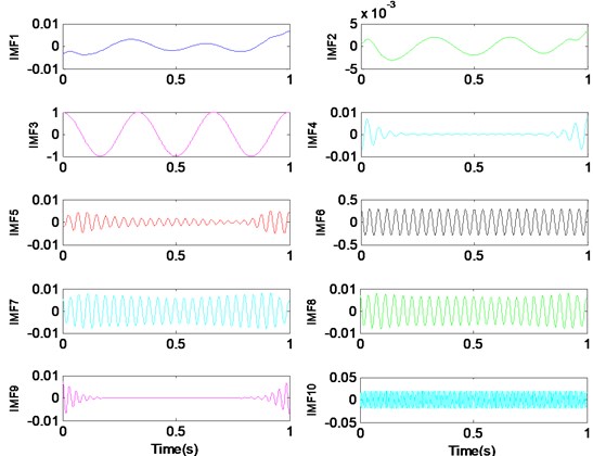
a) VMD , 10
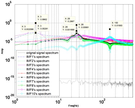
b), 10
From this algorithm, it’s clear that the mode number needs to be given in advance. In order to study the effect of the , we construct a tri-harmonic signal expressed in Eq. (6), which is composed of three different, pure harmonics, whose frequency is 3 Hz, 26 Hz and 150 Hz, respectively:
We set the value of from 1 to 10 to observe decomposition results of the signal. When the preset component number is greater than the actual harmonic number, over-segment of VMD will take place. Fig. 1 illustrates the result of VMD with 10. Fig. 1(a) shows ten modes in time domain and frequency spectrum of these modes are illustrated in the Fig. 1(b). We can learn from Fig. 1(a) that the mode (component) 1, 4, 5 and 9 are incomplete harmonic, which is the result of over-segment. From Fig. 1(b), the center frequency of component 1, 2, 3 are 3 Hz, and the center frequency of mode component 6-8 are 26 Hz, which means that over-decomposition of signal occurs.
When the preset component number is fewer than the actual harmonic number, VMD method will lead to under-segment. The VMD decomposition with 2 (3) is shown in Fig. 2. From Fig. 2(b), VMD separates 150 Hz harmonic signal into two parts, which are added to the signal of 3 Hz and 26 Hz respectively. Too few modes will lead to under-segmentation. Some components are separated and contained in other components, or discarded as “noise”.
Fig. 2Too few modes (K= 2) lead to under-segmentation of the signal
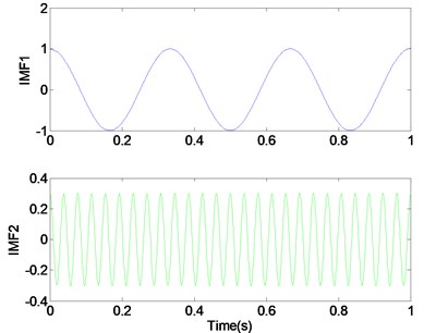
a) VMD , 2
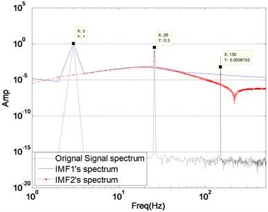
b), 2
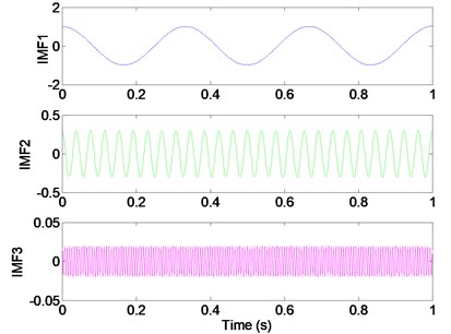
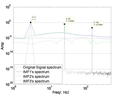
When the preset modes number is the same as the actual component number, VMD of signal can achieve exact tones. Fig. 3 is the decomposition result with 3, and three components are recovered almost flawlessly. Fig. 3(b) are frequency expression of original signal and three components. We can learn from Fig. 3, the center frequency of each component (3 Hz, 26 Hz and 150 Hz) is the same as the center frequency of original signal components, respectively. The amplitude of each component is 1, 0.3 and 0.02, which are consistent with the original signal components.
We can learn from the results of simulation: the value makes a great influence on decomposition, only when is chosen properly. We can get more accurate components from the original signal, without mode overlap and mode duplication. Because number must be given in advance, reasonable pre-estimation of the parameter of VMD is rather important and is of practical significance. An adaptive estimation method will be proposed in the following text.
Fig. 3Appropriate modes (K= 3) lead to correct segmentation of the signal
a) VMD , 3
b), 3
3. Adaptive estimation method of VMD based on cross correlation coefficient
The cross correlation coefficient is used as the statistical indicators of the affinity degree among the different variables [10, 11]. The cross correlation coefficient is calculated by covariance method. Similarly, according to two variables and their average deviation, multiply two average deviations are multiplied to show the relevant degree of two variables. The calculation formula [10] of the cross correlation coefficient between two sequence and is written as:
According to the properties of cross correlation coefficient, if signals and are periodic signal with same frequency or contain periodic components of the same frequency, cross correlation coefficient will be larger. If and have periodic signals with different frequencies, cross correlation coefficient will be smaller. Large amounts of experiments are conducted with from 0.5 to 1.5, When is equal about to 0.1, the effect is most stable, and the result is more consistent with what we have expected. So, we recommend 0.1 as threshold value to judge whether two signals are relevant. In VMD, if cross correlation coefficient between two components is larger than 0.1, we judge that over-segmentation occurs.
In VMD, each component is a part of original signal (). If the cross correlation coefficient between component and original signal is less than the coefficient between component and another component , we can say that the component is much closer to the component than to the original signal. If that situation happens, we also consider that over-segmentation occurs.
Synthetic signal as Eq. (6), is operated by VMD with 10, the cross correlation coefficients among components and the original signal are mentioned in Table 2. From Table 2, the cross correlation coefficients among components 1-3 (, , ) are 0.75, 0.52 and 0.9, so 1-3 should be one component. The cross correlation coefficients among components 5-8 (, , , , , ) are 0.51, 0.67, 0.73, 0.75, 0.94, 0.87, so 5-8 should be one component. Over segmentation occurs when synthetic signal is operated by VMD with 10. The conclusion is consistent with the fore graphic analysis results in Section 2. From Table 2, because and 0.17 > 0.1, component 4 is also the product of over-segmentation, which is also consistent with the situation of component 4 shown in Fig. 1(a).
Table 2The cross correlation coefficient among VMD components and original signal (K = 10)
IMF 1 | IMF2 | IMF3 | IMF4 | IMF5 | IMF6 | IMF7 | IMF8 | IMF9 | IMF10 | Original signal | |
IMF1 | 1 | 0.75 | 0.52 | 0.02 | 0.01 | 0.00 | 0.00 | 0.00 | 0.01 | 0.00 | 0.60 |
IMF2 | 1 | 0.90 | 0.03 | 0.02 | 0.00 | 0.01 | 0.01 | 0.01 | 0.00 | 0.96 | |
IMF3 | 1 | 0.00 | 0.00 | 0.00 | 0.00 | 0.00 | 0.00 | 0.00 | 0.02 | ||
IMF4 | 1 | 0.17 | 0.02 | 0.06 | 0.06 | 0.04 | 0.00 | 0.01 | |||
IMF5 | 1 | 0.51 | 0.67 | 0.73 | 0.11 | 0.00 | 0.22 | ||||
IMF6 | 1 | 0.75 | 0.94 | 0.02 | 0.00 | 0.29 | |||||
IMF7 | 1 | 0.87 | 0.08 | 0.00 | 0.28 | ||||||
IMF8 | 1 | 0.08 | 0.00 | 0.12 | |||||||
IMF9 | 1 | 0.00 | 0.01 | ||||||||
IMF10 | 1 | 0.02 | |||||||||
Original signal | 0.60 | 0.96 | 0.02 | 0.01 | 0.22 | 0.29 | 0.28 | 0.12 | 0.01 | 0.02 |
Then, we focus on the characters of cross correlation coefficient in under-segmentation. After VMD operation of signal as Eq. (7) with 2, the cross correlation coefficients among components and the original signal are shown in Table 3. From Table 3, we can learn that cross correlation coefficient between component 1 and 2 is 0, over-segmentation doesn’t happen, and there are no characters about under-segmentation. How can we judge a suitable ? We can use to operate VMD, then observe whether there exists over-segmentation. If there exists over-segmentation with , the value of is the appropriate estimation. If not, continue to add 1 until the over-segmentation occurs.
Fig. 4flow chart of K adaptive estimation
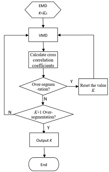
Table 3The cross correlation coefficient among VMD components and original signal (K= 2)
IMF1 | IMF2 | Original signal | |
IMF1 | 1 | 0.00 | 0.96 |
IMF2 | 0 | 1 | 0.29 |
Original signal | 0.96 | 0.29 |
Thus, the estimation algorithm of can be designed as Fig. 4. Firstly, set , operate VMD, calculate the cross correlation coefficients among components and the original signal, and judge whether it is over-segmented. If it is over-segmented, calculate the numbers of over-segmentation, subtract the numbers, reset the value of and return to VMD. Otherwise, judge whether is over-segmented. If is over-segmented, the value is what we want.
The variational mode decomposition (VMD) proposed recently has obvious advantages on signal decomposition such as high precision and noise robustness, but its number of modes () must be given in advance. Now, the mode number can only be estimated by prior knowledge. And if chosen inappropriately, it will lead to larger decomposition error. As a result, we focus on the research of the over- and under-segment characters of VMD. The estimation method of VMD parameter is proposed based on cross correlation coefficients among VMD components and the original signal. The method is proved feasible and effective through analyzing simulation signals and extracting the fault feature of rolling bearing.
The Hilbert-Huang transform (HHT) is an adaptive time-frequency method which was developed by Huang in 1998. The HHT method has two steps, empirical mode decomposition (EMD) and Hilbert spectral analysis (HSA) [11-14]. The EMD, the first step, is to decompose the data into finite different intrinsic mode function (IMF) components, which represents different oscillatory modes and acts as a pre-processor for HSA. Based on the local extrema, the EMD method provides an adaptive method for decomposition of signals. Because the IMF components are decomposed adaptively, its number is associated with real modes of signal and can be used as the initial (), thus avoiding giving an initial value blindly.
4. Adaptive estimation of simulation signal
4.1. Adaptive estimation of non-noise simulation signal
Now, we estimate the value of for non-noise simulation signal like Eq. (6). According to Fig. 4, firstly, operate EMD and we can get 3 IMFs. So, we set 3, then operate VMD with 3 and calculate the cross correlation coefficients shown in Table 4, from which we can know it isn’t over-segmented. As a result, we set 4 and go back to the VMD. Similarly, calculate again the cross correlation coefficients shown in Table 5. Obviously, over-segmentation appears, so the value 3 is the last output of algorithm. Compared to the actual signal, the estimated value (3) is suitable.
Table 4The cross correlation coefficients for tri-harmonic signal (K= 3)
IMF1 | IMF2 | IMF3 | Original signal | |
IMF1 | 1 | 0.00 | 0.00 | 0.96 |
IMF2 | 0 | 1 | 0.00 | 0.29 |
IMF3 | 0 | 0 | 1 | 0.0200 |
Original signal | 0.96 | 0.29 | 0.02 |
Table 5The cross correlation coefficients for tri-harmonic signal (K= 4)
IMF1 | IMF2 | IMF3 | IMF4 | Original signal | |
IMF1 | 1 | 0.00 | 0.00 | 0.00 | 0.96 |
IMF2 | 0 | 1 | 1.00 | 1.00 | 0.29 |
IMF3 | 0 | 0 | 1 | 1.00 | 0.29 |
IMF4 | 0 | 0 | 0 | 1 | 0.29 |
Original signal | 0.96 | 0.29 | 0.29 | 0.29 |
4.2. Adaptive estimation of noise simulation signal
To estimate the value with noise signal, we use the following tri-harmonic signal affected by noise:
where represents the Gaussian additive noise, and controls the noise level (standard deviation). Here we pick .
According to our algorithm shown in Fig. 4, perform EMD operation first and 5 IMFs are obtained, so 5. The all cross correlation coefficients after VMD operation with 5 are shown in Table 6. The coefficient between component 4 and 5 is higher than the one between component 5 and the original signal. So there exists one over-decomposition and is set to be 4 (). So, we continue to operate VMD with 4 and the cross correlation coefficients are shown in Table 7. Every coefficient is less than 0.1, so over-segmentation doesn’t appear. And we know, when 5, the decomposition is over-segmented, so the final output is 4.
Table 6The cross correlation coefficients for noisy tri-harmonic signal (K= 5)
IMF1 | IMF2 | IMF3 | IMF4 | IMF5 | Original signal | |
IMF1 | 1 | 0.00 | 0.00 | 0.00 | 0.00 | 0.95 |
IMF2 | 1 | 0.00 | 0.00 | 0.00 | 0.29 | |
IMF3 | 1 | 0.02 | 0.01 | 0.07 | ||
IMF4 | 1 | 0.08 | 0.06 | |||
IMF5 | 1 | 0.06 | ||||
Original signal | 0.95 | 0.29 | 0.07 | 0.06 | 0.06 |
Table 7The cross correlation coefficients for noisy tri-harmonic signal (K= 4)
IMF1 | IMF2 | IMF3 | IMF4 | original signal | |
IMF1 | 1 | 0.00 | 0.00 | 0.00 | 0.96 |
IMF2 | 1 | 0.00 | 0.00 | 0.29 | |
IMF3 | 1 | 0.02 | 0.04 | ||
IMF4 | 1 | 0.03 | |||
original signal | 0.96 | 0.29 | 0.04 | 0.03 |
However, we know that this signal contains tri-harmonic. Let’s observe what will happen with 3. Perform VMD with 3, then calculate all the cross correlation coefficients shown in Table 8. According to the data, the decomposition can be judged not over-segmented. However, when 3, the three extracted frequency centers are 3 Hz, 26 Hz and 359 Hz. The original harmonic of 150 Hz is not drawn out and is combined with the noise.
When 4, the four extracted frequency centres are 3 Hz, 26 Hz, 150 Hz, 318 Hz. The three original harmonics of 3 Hz, 26 Hz and 150 Hz are all drawn out and the rest component of 318 Hz can be considered as noise. 4 is more reasonable.
Table 8The cross correlation coefficients for noisy tri-harmonic signal (K= 3)
IMF1 | IMF2 | IMF3 | Original signal | |
IMF1 | 1 | 0.00 | 0.00 | 0.95 |
IMF2 | 0 | 1 | 0.00 | 0.30 |
IMF3 | 0 | 0 | 1 | 0.06 |
Original signal | 0.95 | 0.30 | 0.06 |
4.3. Adaptive estimation for rolling bearing fault signal
Rolling element bearing fault data is obtained from the Case Western Reserve University Bearing Data Centre. The experimented bearing is 6205-2RS JEM SKF, deep groove ball bearing. The rotating speed is 1730 rpm and the sampling frequency is 12 kHz. Three experiments conducted are inner raceway, ball and outer raceway fault signal decomposition, respectively. Now we only discuss the inner raceway fault signal decomposition in detail. The theoretical fault feature frequency of inner raceway is 156.1 Hz.
First, perform EMD operation to get the initial . After EMD operation, 12 IMFs can be obtained. The initial value of is 12 and the cross correlation coefficients after VMD operation with 12 are shown in the Table 9. There are 6 cross correlation coefficients higher than or equal to 0.1, so is reset as 6 ().
Then operate VMD with 6 and the cross correlation coefficients are shown in the Table 10. There is 1 cross correlation coefficient between 5 and 6 greater than 0.1, so is reset as 5 (). Then, operate VMD with 5 and cross correlation coefficients shown in Table 11 are obtained. From Table 11, we can know that one over-segmentation occurs. Set 4 and operate VMD again. The cross correlation coefficients with 4 shown in Table 12 are obtained. Consequently, there is no over-segmentation. Because the decomposition with 5 is over-segmented, the output is 4.
To verify whether the value is reasonable, a contrastive analysis study is given. The envelop spectrum is often used in rolling bearing fault analysis. Fig. 5 and Fig. 6 illustrate the envelop spectrum of VMD operation with 4 and 5 respectively. The practical fault feature frequency (155.3 Hz) and its double-frequency (310.5 Hz) both appear.
Table 9The cross correlation coefficients for rolling bearing fault signal (K= 12)
IMF1 | IMF2 | IMF3 | IMF4 | IMF5 | IMF6 | IMF7 | IMF8 | IMF9 | IMF10 | IMF11 | IMF12 | Original signal | |
IMF1 | 1.00 | 0.16 | 0.04 | 0.01 | 0.00 | 0.00 | 0.00 | 0.00 | 0.00 | 0.00 | 0.00 | 0.00 | 0.12 |
IMF2 | 1.00 | 0.03 | 0.01 | 0.00 | 0.00 | 0.00 | 0.00 | 0.00 | 0.00 | 0.00 | 0.00 | 0.20 | |
IMF3 | 1.00 | 0.13 | 0.01 | 0.00 | 0.00 | 0.00 | 0.00 | 0.00 | 0.00 | 0.00 | 0.26 | ||
IMF4 | 1.00 | 0.01 | 0.00 | 0.00 | 0.00 | 0.00 | 0.00 | 0.00 | 0.00 | 0.31 | |||
IMF5 | 1.00 | 0.06 | 0.01 | 0.00 | 0.00 | 0.00 | 0.01 | 0.01 | 0.36 | ||||
IMF6 | 1.00 | 0.03 | 0.01 | 0.01 | 0.01 | 0.01 | 0.01 | 0.36 | |||||
IMF7 | 1.00 | 0.13 | 0.04 | 0.03 | 0.03 | 0.01 | 0.34 | ||||||
IMF8 | 1.00 | 0.22 | 0.06 | 0.03 | 0.01 | 0.47 | |||||||
IMF9 | 1.00 | 0.10 | 0.03 | 0.01 | 0.51 | ||||||||
IMF10 | 1.00 | 0.11 | 0.01 | 0.39 | |||||||||
IMF11 | 1.00 | 0.04 | 0.20 | ||||||||||
IMF12 | 1.00 | 0.08 | |||||||||||
Original signal | 0.12 | 0.20 | 0.26 | 0.31 | 0.36 | 0.36 | 0.34 | 0.47 | 0.51 | 0.39 | 0.20 | 0.08 |
Table 10The cross correlation coefficients for rolling bearing fault signal (K= 6)
IMF1 | IMF2 | IMF3 | IMF4 | IMF5 | IMF6 | Original signal | |
IMF1 | 1 | 0.08 | 0.02 | 0.01 | 0.00 | 0.00 | 0.23 |
IMF2 | 1 | 0.07 | 0.01 | 0.00 | 0.00 | 0.37 | |
IMF3 | 1 | 0.03 | 0.00 | 0.00 | 0.37 | ||
IMF4 | 1 | 0.00 | 0.00 | 0.37 | |||
IMF5 | 1 | 0.11 | 0.48 | ||||
IMF6 | 1 | 0.66 | |||||
Original signal | 0.23 | 0.37 | 0.37 | 0.37 | 0.48 | 0.66 |
Table 11The cross correlation coefficients for rolling bearing fault signal (K= 5)
IMF1 | IMF2 | IMF3 | IMF4 | IMF5 | Original signal | |
IMF1 | 1 | 0.04 | 0.01 | 0.00 | 0.00 | 0.23 |
IMF2 | 0 | 1 | 0.17 | 0.01 | 0.00 | 0.38 |
IMF3 | 0 | 0 | 1 | 0.06 | 0.02 | 0.46 |
IMF4 | 0 | 0 | 0 | 1 | 0.02 | 0.49 |
IMF5 | 0 | 0 | 0 | 0 | 1 | 0.68 |
Original signal | 0.23 | 0.38 | 0.46 | 0.49 | 0.68 |
Table 12The cross correlation coefficients for rolling bearing fault signal (K= 4)
IMF1 | IMF2 | IMF3 | IMF4 | Original signal | |
IMF1 | 1 | 0.04 | 0.01 | 0.00 | 0.24 |
IMF2 | 1 | 0.02 | 0.01 | 0.38 | |
IMF3 | 1 | 0.04 | 0.50 | ||
IMF4 | 1 | 0.74 | |||
Original signal | 0.24 | 0.38 | 0.50 | 0.74 |
Fig. 5Envelop spectrums of each component after VMD operation with K= 4
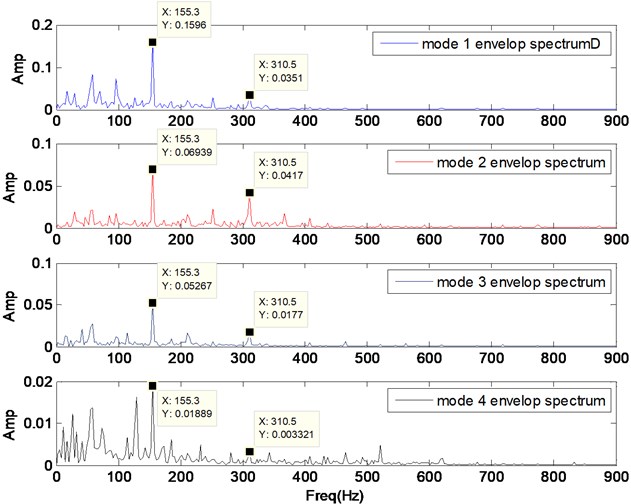
Fig. 6Envelop spectrums of each component after VMD operation with K= 5
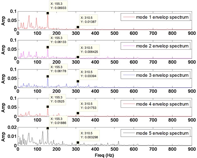
In both pictures (Figs. 5, 6), all the 155.3 Hz character frequency are prominent. Double-frequency amplitudes of component 4 and 5 in Fig. 6 are similar to the ones of component 3 and 4 in Fig. 5. Also, double-frequency amplitude of component 2 in Fig.6 is very weak, only 0.006. And from Table 11, the cross correlation coefficient between component 2 and 3 is 0.17, which is higher than 0.1. Thus, the component 2 in Fig. 6 can be considered as over-segmented from component 3. Therefore, 4 is more suitable than 5.
5. Conclusions
As a newly proposed time-frequency analysis method, VMD performs better performance in tone detection, tone separation and noise robustness. However, the result of the VMD is sensitive to the modes number . VMD over-segment and under-segment have been discussed, and cross correlation coefficients among modes and original signal have been analyzed. We build a relationship between the over-segmentation and cross correlation coefficients, on which the proposed estimation method of VMD Parameter is based. In the algorithm, the initial value of is determined by the numbers of IMFs by EMD. The method is proved feasible and effective by analyzing simulation signals and extracting the fault feature of rolling bearing.
References
-
Wang G. B., He Z. J., Chen X. F., Lai Y. N. Basic research on machinery fault diagnosis – what is the prescription. Journal of Mechanical Engineering, Vol. 49, Issue 1, 2013, p. 63-72.
-
Yayli Mustafa Ozgur On the axial vibration of carbon nanotubes with different boundary conditions. Micro and Nano Letters, Vol. 9, Issue 11, 2014, p. 807-811.
-
Yayli Mustafa Ozgur Free vibration behavior of a gradient elastic beam with varying cross section. Shock and Vibration, Vol. 2014, 2014.
-
Dragomiretskiy K., Zosso D. Variational mode decomposition. IEEE Transactions on Signal Processing, Vol. 62, Issue 3, 2014, p. 531-544.
-
Tang Guiji, Wang Xiaolong Parameter optimized variational mode decomposition method with application to incipiant fault diagnosis of rolling bearing. Journal of Xi’an Jiaotong University, Vol. 49, Issue 5, 2015, p. 73-81.
-
Liu Changliang, Wu Yingjie, Zhen Chengang Rolling bearing fault diagnosis based on variational mode decomposition and fuzzy C means clustering. Proceeding of the CSEE, Vol. 35, Issue 13, 2015, p. 3358-3365.
-
An Lian-suo, Feng Qiang, et al. Variational mode decomposition and its application to monitor the furnace pressure pipeline weak signal detection of leakage. Boiler Technology, Vol. 46, Issue 4, 2015, p. 1-6.
-
Yin Aijun, Ren Hongji A propagating mode extraction algorithm for microwave waveguide using variational mode decomposition. Measurement Science and Technology, Vol. 46, 2015, p. 1-10.
-
Wang Yanxue, Markert Richard, Xiang Jiawei, Zhang Weiguang Research on variational mode decomposition and its application in detecting rub-impact fault of the rotor system. Mechanical System and Signal Processing, Vols. 60-61, 2015, p. 243-251.
-
Ding Chang-Fu, Cai Zhi-Cheng Methods of selecting valid IMF in EMD. Thermal Power Generation, Vol. 43, Issue 1, 2014, p. 36-40.
-
Meng Lingjie, Xiang Jiawei, Wang Yanxue, et al. A hybrid fault diagnosis method using morphological filter-translation invariant wavelet and improved ensemble empirical mode decomposition. Mechanical Systems and Signal Process, Vol. 50, Issue 51, 2015, p. 101-115.
-
Norden E., Huang Z. S., et al. The empirical mode decomposition and the Hilbert spectrum for nonlinear and non-stationary time series analysis. Proceedings of the Royal Society of London A, Vol. 454, 1998, p. 903-995.
-
Huang N. E. A new view of nonlinear waves: the Hilbert spectrum. Annual Review of Fluid Mechanics, Vol. 31, 1999, p. 417-457.
-
Peng Z. K., Tse Peter W., Chu F. L. A comparison study of improved Hilbert-Huang transform: Application to fault diagnosis for rolling bearing. Mechanical Systems and Signal Process. Vol. 19, Issue 5, 2055, p. 974-988.
