Abstract
A method based on ensemble empirical mode decomposition (EEMD), base-scale entropy (BSE) and clustering by fast search (CFS) algorithm for roller bearings faults diagnosis is presented in this study. Firstly, the different vibration signals were decomposed into a number of intrinsic mode functions (IMFs) by using EEMD method, then the correlation coefficient method was used to verify the correlation degree between each IMF and the corresponding original signals. Secondly, the first two IMF components were selected according to the value of correlation coefficient, each IMF entropy values was calculated by BSE, permutation entropy (PE), fuzzy entropy (FE) and sample entropy (SE) methods. Thirdly, comparing the elapsed time of BSE/PE/FE/SE models, using the first two IMF-BSE/PE/FE/SE entropy values as the input of CFS clustering algorithm. The CFS clustering algorithm did not require pre-set the number of clustering centers, the cluster centers were characterized by a higher density than their neighbors and by a relatively large distance from points with higher densities. Finally, the experiment results show that the computational efficiency of BSE model is faster than that of PE/FE/SE models under the same fault recognition accuracy rate, then the effect of fault recognition for roller bearings is good by using CFS method.
1. Introduction
The major electric machine faults include bearing defects, stator faults, broken rotor bar and end ring, and eccentricity-related faults. The failure of rolling element bearings can result in the deterioration of machine operating conditions. Therefore, it is significant to detect the existence and severity of a fault in the bearing fast accurately and easily. Owing to vibration signals carry a great deal of information representing mechanical equipment health conditions, the use of vibration signals is quite common in the field of condition monitoring and diagnostics of rotating machinery [1-4]. Actually, roller bearings fault diagnosis is a pattern recognition process, which includes acquiring information, extracting features and recognizing conditions. The latter two are key links.
On one hand, the purpose of extracting features is to extract parameters representing the machine operation conditions to be used for machine condition identification. Since the characteristics of rolling bearing fault signals are nonlinear and non-flat stability. Feature extraction based on nonlinear dynamics parameters such as fractal dimension, approximate entropy (AE), sample entropy (SE), fuzzy entropy (FE) and permutation entropy (PE) have been applied to the mechanical fault diagnosis, and it has become one of the new ways of nonlinear time series analysis. Pincus M. proposed the AE method and applied it into fault diagnosis [5, 6]. However, the effect of AE method depends on the length of the data heavily. As a result, the value of AE is uniformly lower than the expected one and lacks relative coherence especially when the data length is short. To overcome this drawback, Richman J. S. and Moorman J. R. proposed a new SE method [7], in which SE was applied in the fault diagnosis of mechanical failure successfully [8]. Nonetheless, the similarity definition of AE and SE is based on the heaviside step function, which is discontinuous and mutational at the boundary. As a substitute for improvement, fuzzy entropy (FE) has been proposed by Chen W. T. et al. recently [9, 10], it has been widely applied in medical physiology signal processing and mechanical fault diagnosis [11]. Permutation entropy (PE) was presented by Bandit C. and Pompe B. [12], for the complexity analysis of time domain data by using the comparison of neighboring values. It is reported that for some well-known chaotic dynamical systems, PE performs similar to Lyapunov exponents. The advantages of PE are its simplicity, fast calculation, robustness, and invariance with respect to nonlinear monotonous transformations [12], it has been successfully applied in mechanical fault diagnosis [13-15]. However, the SE and FE methods need increase the dimension m to m+1 for constructing the vector set sequences Xi [6-11], and calculate the number of vector Bm(r) and Bm+1(r) (here r is similarity tolerance in SE and FE methods) with the distance dij between two vectors Xi and Xj. In PE method, it needs to sort each matrix Xi with m dimension when calculating the probability Pi distribution of each symbol m-dimensional sequences Xi. A method named base-scale entropy (BSE) proposed in reference [16]. It did not like the PE/FE/SE methods which need complicated sorting operation, the BSE makes only use all the adjacent points by using the root mean square in m-dimensional vector Xi to calculating the base-scale(BS) value [16], this method is simplicity and extremely fast calculation to short data sets, it was applied in physiological signal processing [17].
The commonly used signal decomposing method includes wavelet analysis [18, 19], empirical mode decomposition (EMD) [20], etc. However, wavelet transform requires choosing wavelet basis and decomposing layers, which makes it a non-adaptive signal processing method in nature. EMD method can decompose a complex signal self-adaptively into some intrinsic mode functions (IMFs) and a residual. To overcome the problem of mode mixing in EMD, ensemble empirical mode decomposition(EEMD) [21], an improved version of EMD, can self-adaptively decompose a complicated signal into IMFs based on the local characteristic timescale of the signal. Recently, EEMD has been widely applied in fault diagnosis [13, 22]. Considering that the IMFs decomposed by EEMD represent the natural oscillatory mode embedded in the signal, the BSE values of each IMF (IMF-BSE) are extracted as feature vector to reveal the characteristics of the vibration signals.
After extracting the feature parameters with EEMD and BSE, naturally, a classifier is expected to achieve the rolling bearing fault diagnosis automatically, such as support vector machine (SVM) [23] with particle swarm optimization (PSO) algorithm [24] and neural network (NN), label data sets are assumed available. But in practical applications, the data sets are usually unlabeled. Fuzzy c-means (FCM) algorithm [25] is a common method for rolling bearing fault diagnosis when the data is unlabeled [26]. FCM algorithm is suitable for data structure with the homogenous structure, but it can only handle the spherical distance data of the standard specification. Gustafson-kessel (GK) clustering algorithm is an improved FCM algorithm, in which adaptive distance norm and covariance matrix are introduced. As GK can handle subspace dispersion and scattering along any direction of the data [27], GK cluster has been successfully used in fault diagnosis [28]. As the Euclidean distance is used to compute the distance between two sample in FCM and GK algorithms, hence they are only handle data with a sphere-like structure. Since the distribution patterns of the data are seldom spheres, gath-geva (GG) clustering algorithm is proposed for this purpose [29]. Fuzzy maximum likelihood estimation of distance norm can reflect the different shape and orientations of data structure [30]. Most clustering methods such as FCM, GK and GG clustering algorithms require pre-determining the number of clustering centers which decides the clustering accuracy. To solve this problem, a method called clustering by fast search (CFS) algorithm which did not require pre-set the number of clustering centers is proposed in [31]. The CFS algorithm is aimed at classifying elements into categories on the basis of their similarity, the cluster centers are characterized by a higher density than their neighbors and a relatively large distance from points with higher densities.
As mentioned above, combining EEMD, BSE and CFS, an intelligent fault detection and classification method for fault diagnosis of roller bearings is presented with experimental validation. Firstly, using the EEMD method to decompose the vibration signals under different conditions into a number of IMFs. Secondly, calculating the correlation coefficient value between each IMF component and the corresponding original signal. Using the BSE/PE/FE/SE methods to calculate the IMFs entropy values, then comparing the elapsed time of BSE/PE/FE/SE methods, respectively. Finally, selecting the first two IMFs entropy values according to the value of correlation coefficients as the input of CFS clustering model for fulfill the fault recognition. The experiment results show that the computational efficiency of BSE model is faster than PE/FE/SE models under the same classification accuracy.
The rest of this paper is organized as follows: Section 2 presents the review of EEMD, BSE and CFS models, respectively. Section 3 gives fault diagnosis methodology. Section 4 describes the experimental data sources and parameters selection for EEMD, BSE, PE, FE, SE and CFS models. Experiments validation is given in Section 5 followed by conclusions in Section 6.
2. Review of EEMD, BSE and CFS
2.1. Theoretical framework of EEMD
EEMD [13, 21, 22] is a substantial improvement method of EMD [20], and its procedures are as follows:
Step 1: Given that X(t) is an original signal, add a random white noise signal nj(t) to X(t):
where Xj(t) is the noise-added signal, j=1, 2, 3,…, m and m is the number of trial.
Step 2: The original signals X(t) are decomposed into a number of IMFs by using EMD as follows:
where cij indicates that the ith IMF of the jth trial uNj describes the residue of jth trial, and N is the IMFs number of the jth trial.
Step 3: If j<m, then repeat step1 and step 2, and add different random white noise signals each time.
Step 4: Obtain that I=min(N1,N2,…,Nm) and calculate the ensemble means of the corresponding IMFs of the decompositions as the final result:
where i=1, 2, 3,…, I.
Step 5: ci (i=1, 2, 3,…, I) is the ensemble mean of corresponding IMF of the decompositions.
2.2. Theoretical framework of BSE
The mathematical theorem of the BSE was described in detail in reference [16, 17]. The steps for BSE can be described as follows:
Step 1: Considering a time series u of N points as follows: {u|u1,u2,⋅⋅⋅,ui,1≤i≤N} for given m. The dataset sequences {Xmi|Xm1,Xm2,⋅⋅⋅Xmi,1≤i≤N-m+1} are constructed in a form as:
where Xmi indicates m consecutive u values, so it has a number of N-m+1 vectors with m-dimension.
Step 2: Base-scale (BS) is defined as the root mean square under difference value of all adjacent points in m-dimensional vector Xmi. The BSE value of each m-dimensional vector Xmi is calculated as follows:
Step 3: Each m-dimensional vector Xmi is transformed into a symbol vector set sequences Si(X(i))={s(i),⋅⋅⋅,s(i+m-1)},s∈A(1,2,3,4). The symbol dividing standard is chosen as a*BS. Therefore, procedure for Si(X(i)) with m-dimension is given as:
where i=1, 2,…, N-m+1, k= 1, 2,…, m-1, the meaning of ¯u and a are the average value of the ith vector Xmi and a constant respectively. The symbol set sequences {1, 2, 3, 4} are just label which is used to statistical probability distribution for each vector Xmi, they have not make any sense.
Step 4: The probability distribution P(π) is calculated for each vector Si(X(i)). Therefore, there are 4m different composite states π in Si(X(i)) and each state represents a different mode. The calculation of P(π) is given as follows:
where 1≤t≤N-m+1.
Step 5: The BSE is defined as:
2.3. Theoretical framework of CFS clustering
CFS clustering algorithm uses the value of density and distance between two points to determine the clustering centers. The steps for CFS method [31] can be described as follows:
Step 1: For a given data set with N points X={x1,x2,…,xN}, the distance of two points xi and xj as follows:
where m is the dimension of each point.
Step 2: Computing the local density ρi of each point:
where ρi is equal to the number of points that are closer than cutoff distance dc to point i.
Step 3: The parameter δqi is measured by computing the minimum distance between the point i and other points with higher density:
where {qi}Ni=1 is a descending order subscript of the local density {ρi}Ni=1. Note that δqi is much larger than the typical nearest neighbor distance only for points that are local or global maximum in the density.
Step 4: Using the value of γ to determine the clustering centers:
The larger value of γi, the more possibility of the point i become a clustering center, here the value of γ is in descending order.
Step 5: Computing the number of data points for each clustering center point according to the cutoff distance dc.
3. Procedures of the proposed method
An intelligent fault diagnosis strategy, which is based on EEMD, BSE and CFS models, is proposed in this study. Procedure of the proposed system can be summarized as follows:
Step 1: Preprocessing vibration signals under different conditions are decomposed into a number of IMFs by using EEMD model. The original signals are decomposed into a series of IMFs, but the first IMF is the highest frequency portion of the original signals, and other IMFs in descending order, therefore, the first two IMFs contains the main information of the original signals.
Step 2: Calculating the correlation coefficient value between each IMF and the corresponding original signals. It reduces information redundancy
Step 3: Using the BSE/PE/FE/SE models to calculate the IMF-BSE/PE/FE/SE values, comparing the elapsed time of BSE/PE/FE/SE models, respectively.
Step 4: In order to make the data visualization and improve computational efficiency, then using the first two IMF-BSE/PE/FE/SE entropy values as the input of CFS method.
Step 5: Unlike FCM/GK/GG clustering models, the CFS algorithm which did not require pre-set the number of clustering centers, the cluster centers are characterized by a higher density. and relatively large distance. Using the classification accuracy to compare the EEMD-BSE/PE/FE/SE-CFS models.
Fig. 1 shows the structure of the proposed fault diagnosis method.
4. Experimental data sources and parameter selection
4.1. Rolling bearing data set
In this subsection the proposed approach is applied to the experimental data, which comes from the Case Western Reserve University Bearing Data [32]. Experiment data was collected using accelerometers mounted at the drive end (DE) and fan end (FE) of an induction motor. The motor bearings under consideration were seeded with faults by electro-discharge machining (EDM). Three single point defects (inner race fault (IRF), outer race fault (ORF) and ball fault (BF)) with fault diameters 0.1778 mm in. was introduced separately. The fault seeded at the outer race was placed at a position equivalent to 6:00 o’clock time configuration. The data collection system consists of a high bandwidth amplifier particularly designed for vibration signals and a data recorder with a sampling frequency of 12,000 Hz per channel. Table 1 shows the working conditions considered in this study. In Table 1, “NR” denotes the bearings with no faults and “BF”, “IRF” and “ORF” denote the ball fault in ball, inner race fault and outer race fault. 0.1778 mm is the fault diameters. The motor revolving speed was chosen as 1,750 rpm from the drive end of the motor.
Fig. 1Flow chart of the proposed method
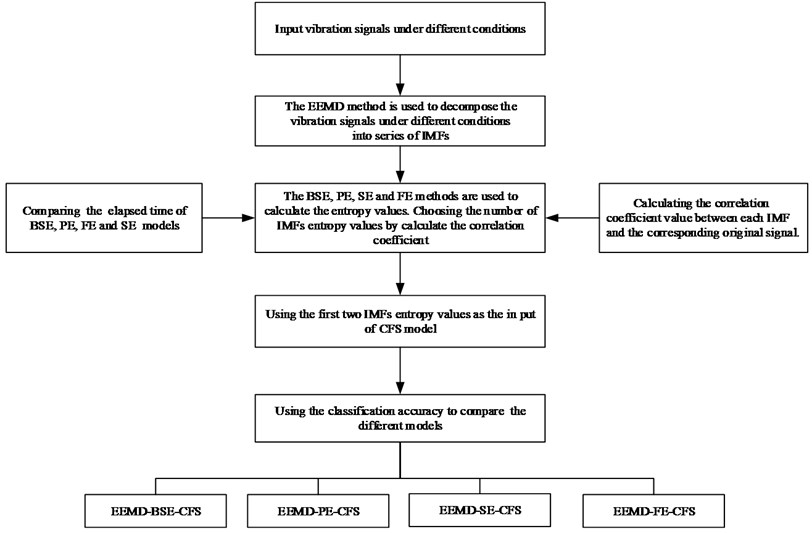
Table 1The rolling bearing experimental data under different conditions
Fault category | Fault diameters (mm) | Motor speed (rpm) | Number of samples |
NR | 0 | 1750 | 50 |
IRF | 0.1778 | 1750 | 50 |
BF | 0.1778 | 1750 | 50 |
ORF | 0.1778 | 1750 | 50 |
4.2. Parameter selection for different methods
(1) EEMD: EEMD has two parameters to be set, which are the ensemble number m and the amplitude of the added white noise ni(t) in Eq. (1). Generally speaking, an ensemble number of a few hundred will lead to an exact result, and the remaining noise would cause less than a fraction of one percent of error if the added noise has the standard deviation that is a fraction of the standard deviation of the input signal. For the standard deviation of the added white noise, it is suggested to be about 20 % of the standard deviation of the input signal [13]. The parameter m was set as 100.
(2) BSE: The parameter m in Eq. (4) often varies from 3 to 7 [16, 17]. However, too large m value is unfavorable for the need of a very large N≥4m, which is hard to meet generally and will lead to the losing of information. The parameter a in Eq. (3) is a constant. Typically, the parameter a is often fixed as 0.1-0.4 [16, 17], larger a allows more detailed reconstruction of the dynamic process. However, smaller a will be affected by noise. In this paper, the parameters a, and m is set as 0.2, 0.3 and 4, 5, respectively [16, 17].
(3) PE: There are few parameters affect the PE value calculation, such as embedded dimension m and the time delay t. In t Bandit C and Pompe B [12]’s studies, they recommended to select embedded dimension m=3-7 [13-15]. For practical calculation, when m<3, PE cannot detect the dynamic changes of the mechanical vibration signals exactly. On the other hand, when m>8, reconstruction of phase space will homogenize vibration signals, and PE is not only computationally expensive but also cannot be observed easily because of its small varying range. When time delay t>5, the computational results can not exactly detect small changes in signals. The time delay t has a small influence on the PE calculation of the time series [13]. Therefore, in this study, the parameters m, and t is set as 4, 5, 6 and 1 respectively to calculate the PE values of vibration signals.
(4) SE and FE: Three parameters must be selected and determined before the calculation of SE and FE. The first parameter embedding dimension m, as in SE and FE, is the length of sequences to be compared. Typically, larger m allows more detailed reconstruction of the dynamic process [7, 13, 30]. But a too large m value is unfavorable due to the need of a too large N=10m-30m, which is hard to meet generally and will lead to the losing of information. Generally speaking, m is often fixed as 2 [7, 13, 33]. The parameters similarity tolerance r and n determine the width and the gradient of the boundary of the exponential function respectively. In terms to the FE similarity boundary determined by r and n, too narrow settings will result in salient influence from noise, while too broad a boundary, as mentioned above, is supposed to be avoided for fear of information loss. It is convenient to set the width of the boundary as r multiplied by the standard deviation (SD) of the original dataset. Experimentally, r=(0.1-0.25)×SD [7, 10, 11, 33], the parameter r is set as 0.2SD in SE and FE in this paper. Finally, the parameter n is often fixed to 2 [7, 10, 11, 33].
(5) CFS: The parameter cutoff distance dc to be set, as suggested in [31], a cutoff distance dc equals to the average number of neighbors is often set as 1 % to 2 % of the total number of points in the data set [31]. Large dc will lead to the value of local density ρi of each point become high. However, a too small dc value will unfavorable lead to a cluster divided into many clusters. As a result, the parameters dc is set as 1.5 % in this paper.
5. Experimental result s and analysis
The data is selected from the experiments in which SKF bearings are used. The approximate motor speed is 1,750 rpm. The data set consists of 200 data samples in total, 50 data samples under each fault condition and every data sample has 2048 data points. The number of each sample is set as: NR:1-50, IRF: 51-100, BF:101-150, ORF:151-200. As limited space, here with a sample of each state for an example, the time domain waveforms of vibration signals under different working conditions are shown in Fig. 2.
The vertical axis is the acceleration vibration amplitude. Because of the influence of noise, it is difficult to find significant differences in different states. As shown in Fig. 2, it is hard to distinguish the four signals, especially, there is no obvious regularity in two states of NR and BF signals.
After EEMD decomposition, the original signals in Table. 1 are decomposed into IMF1-IMF10 and a residue u, Fig. 3 shows the EEMD decomposition results of the vibration signals, they contain 10 IMF components and a residue u.
Fig. 2The time domain waveforms of each working condition
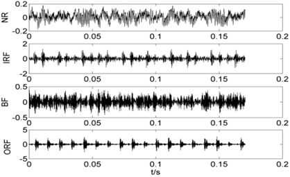
Fig. 3The results of IMFs for different signals by using EEMD method
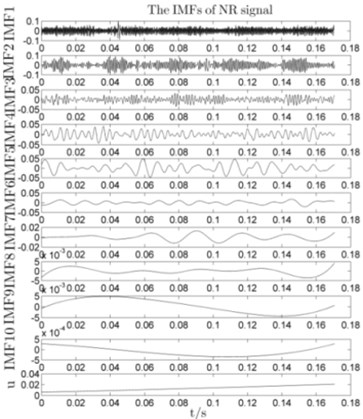
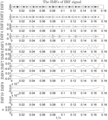
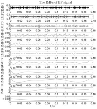
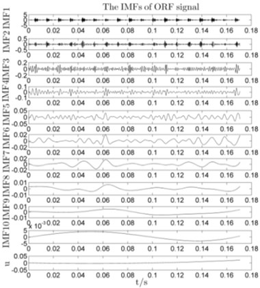
As shown in Fig. 3, IMF1-IMF10 represents a different component from high to low frequency of the original signals, therefore, the first IMF is the highest frequency in all the IMF components. The correlation coefficient method is used to verify the relevance between each IMF and the corresponding original signals, the correlation values of each IMF are given in Table.2 (As limited space, here with a sample of each state for an example).
Table 2The correlation values of each IMF
Mode | IMF1 | IMF2 | IMF3 | IMF4 | IMF5 | IMF6 | IMF7 | IMF8 | IMF9 | IMF10 | |
The value of correlation coefficient | NR | 0.5632 | 0.6771 | 0.4179 | 0.3904 | 0.4336 | 0.2547 | 0.1415 | 0.0436 | 0.0067 | 0.0178 |
IRF | 0.8824 | 0.4346 | 0.2677 | 0.1168 | 0.0412 | 0.0307 | 0.0032 | 0.0001 | 0.0005 | –0.0001 | |
BF | 0.9585 | 0.2083 | 0.1899 | 0.1225 | 0.0780 | 0.0462 | 0.0059 | 0.0046 | 0.0021 | 0.0010 | |
ORF | 0.9858 | 0.1248 | 0.0675 | 0.0304 | 0.0106 | 0.0044 | 0.0006 | 0.0004 | 0.0005 | 0.00001 |
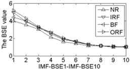
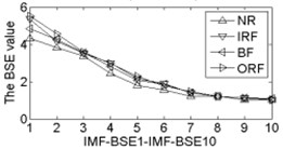
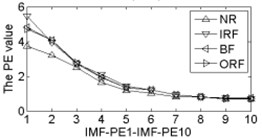
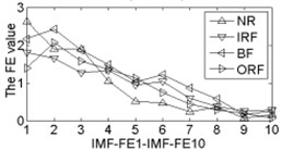
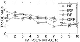
As shown in Table 2, the correlation values of first two IMF components are higher than the other components, it contains the main information of the original signals. Calculating each IMF entropy values by using BSE, PE, FE and SE models, the results of the IMF-BSE/PE/FE/SE values of the corresponding IMFs are shown in Fig. 4.
Fig. 4The BSE, PE, SE and FE values curve
a) BSE (m= 4, a=0.2)
b) BSE (m=4, a=0.3)
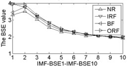
c) BSE (m=5, a=0.2)
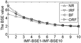
d) BSE (m=5, a=0.3)
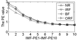
e) PE (m=4)
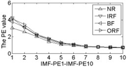
f) PE (m=5)
g) PE (m=6)
h) FE (r=0.2SD)
i) SE (r=0.2SD)
As shown in Fig. 4, the first two IMF-BSE/PE/FE/SE entropy values are higher than the other IMF components, that is because the EEMD method decompose the original signals into high frequency and low frequency components in descending order, the entropy value of the first two IMFs are higher than the other IMFs. Compared with the IMF-SE values, the decreasing tendency of IMF-BSE/PE/FE values are clear on the whole, because the SE method uses the hard threshold r to measure the similarity of m-dimensional vector Xmi and Xmj. The FE introduced the fuzzy exponential functions to measure the similarity and make the signal become smooth, but the smoothing feature of the IMF-FE entropy values are no better than PE and BSE methods, the BSE/PE methods count up the number of probability P(π) for each m-dimensional vector Xmi before compute the BSE and PE entropy values, the original signals are decomposed into a series of IMFs by using EEMD model in descending order. Therefore, the number of probability P(π) for each m-dimensional vector Xmi is close to a fixed value for each IMF, hence the characteristics of continuous and smooth in BSE and PE are better than FE/SE models. The SE and FE methods make use of the d[Xmi,Xmj] smaller than similar tolerance r (SE) and fuzzy exponential (FE) functions to compute the corresponding entropy values, so the characteristics of random mutation exists in the IMF-FE/SE entropy values, it is consistent with the case of Fig. 4(h) and Fig. 4(i), this indicates that the BSE/PE methods can detect small changes in the signal. However, the computational efficiency of BSE model is faster than PE model, the elapsed time of all samples calculated by BSE, PE, FE and SE are counted, which is given in Table 3.
Table 3The elapsed time of each sample by using BSE, PE, FE and SE methods
Mode | The total elapsed time (s) | The average elapsed time (s) |
BSE (m= 4, a=0.2) | 35.338515 | 0.17669258 |
BSE (m=4, a=0.3) | 34.691865 | 0.17345932 |
BSE (m=5, a=0.2) | 53.012515 | 0.26506258 |
BSE (m=5, a=0.3) | 51.799329 | 0.25899664 |
PE (m=4) | 61.151057 | 0.30575528 |
PE (m=5) | 232.389355 | 1.16194678 |
PE (m=6) | 1469.4152 | 7.347076 |
FE (r=0.2SD) | 30837.6027 | 154.188014 |
SE (r=0.2SD) | 36979.1837 | 184.895918 |
As shown in Table 3, when m=5, a=0.2 the biggest total and average elapsed time in BSE method are 53.0.125515 seconds and 0.26506258 seconds, which is smaller than the PE, FE and SE methods. The reasons why the elapsed time of BSE method is the lowest in Table 3 are listed as follows:
(1) For a given original signal Xi with N points, it has (N-m+1) m-dimensional vector Xmi by reconstruction operation [7,12,16], here m is the embedding dimension in BSE/PE/SE/FE methods. The BSE and PE methods takes the same time to reconstruct the original signals Xi [12, 16], but the SE method requires twice reconstruct operations [7]. Therefore, the elapsed time of the SE method is larger than that of BSE and PE methods.
(2) Firstly, the Eq. (5) is used to calculate the BS value in BSE method, it requires addition, subtraction, multiplication, and division operations, the cycle number of these operations are (m-1)(N-m+1), (m-1)(N-m+1), (m-1)(N-m+1) and (N-m+1), respectively. Secondly, it needs to calculate the mean value of each vector Xmi before the Si(X(i)) computation, the cycle number of addition and division operations are (m-1)(N-m+1), (N-m+1), the following step for Si(X(i)) computation include addition, subtraction, multiplication and comparison (“>”, “<” and “=”) operations, the corresponding cycle number are (N-m+1), (N-m+1), (N-m+1), 6(N-m+1). Then count up the number of probability P(π) for each m-dimensional vector Xmi, there are 4m different composite states π included in vector Si(X(i)) because only four kinds of symbol {1, 2, 3, 4} included in BSE method, the number of comparison and division operations which was used to find the state π included in each m-dimensional vector Xmi are 4m (N-m+1) and (N-m+1). Finally, the Eq. (8) is used to calculate the BSE value, the cycle number of addition, multiplication and logarithm operations are (N-m+1), (N-m+1), (N-m+1).
(3) The steps for PE are described in detail in reference [12-14]. Firstly, the PE method needs to sort the overall adjacent two data points [12-14], it requires comparison operations with m(m-1)(N-m+1) cycles. Then count up the number of probability P(π) for each m-dimensional vector Xmi, there are m! different composite states π included in vector Si(X(i)) [12-14], the number of comparison and division operations which was used to find the state π included in each m-dimensional vector Xmi are(m!)m(N-m+1)and (N-m+1). Finally, computing the PE value, the cycle number of addition, multiplication and logarithm operations are (N-m+1), (N-m+1), (N-m+1).
(4) The steps for SE and FE are described in detail in reference [7-11], computing the distance d[Xmi,Xmj]=maxk∈[1...N-1](|x(i+k)-x(j+k)|) between the vector Xmi and Xmj in SE method, it requires m(N-m)(N-m+1) cycles for subtraction operation, and count up the number of Ai which is meeting the condition d[Xmi,Xmj]≤r [7], here r is the similar tolerance. It requires comparison operation (“<” and “=”) with (N-m)(N-m+1) cycles. The following step is count up the number of Cm(r) [7], the number of addition, multiplication and division operations are (N-m+1), (N-m+1) and (N-m+1). Finally, by increasing the m to m+1 and repeating the previous steps to find Cm+1(r) in the following step, the number of division and logarithm operations for calculate the value in SE method are once [7]. In FE, it was imported the concept and employed the exponential functions exp-(d[Xmi,Xmj]2/r) as the fuzzy function to get a fuzzy measurement of two vectors’ similarity based on SE method [9, 10]. Therefore, the total cycle number of basic operations for FE is close to SE.
As mentioned above, the total number of addition, subtraction, multiplication, division and comparison operations of BSE/PE/SE/FE models are given in Table 4.
It can be seen that the total number of BSE method is (4m+4m+11)(N-m+1), which is smaller than that of the PE/SE method because the parameter m≥2 (here N=2048 in this paper). Therefore, the BSE method is faster than PE/SE methods
Table 4The total number of basic operations of BSE/PE/SE models
Operation | BSE | PE | SE/FE |
+ | 2m(N-m+1) | (N-m+1) | 2(N-m+1) |
– | m(N-m+1) | – | 2m(N-m)(N-m+1) |
* | (m+1)(N-m+1) | (N-m+1) | 2(N-m+1) |
/ | 3(N-m+1) | (N-m+1) | 2(N-m+1)+3 |
log | (N-m+1) | (N-m+1) | 1 |
>, <, = | 6(N-m+1)+4m(N-m+1) | m(m-1)(N-m+1)+(m!)m(N-m+1) | 2(N-m)(N-m+1) |
Total | (4m+4m+11)(N-m+1) | [(m!)m+m2-m+4](N-m+1) | [2(m+1)+(N-m)+4](N-m+1)+4 |
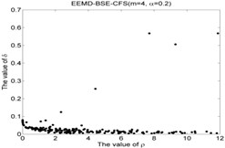
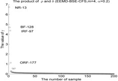
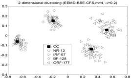
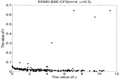
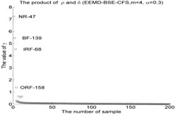
Fig. 5The results of the local density ρ, distance δ, γ and the 2-dimension clustering for all samples
1)
2)
3)
4)
5)
6)
7)
8)
9)
10)
11)
12)
13)
14)
15)
16)
17)
18)
19)
20)
21)
22)
23)
24)
25)
26)
27)
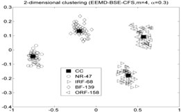
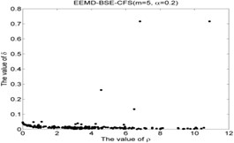
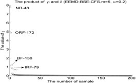
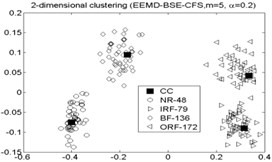
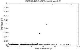
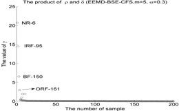
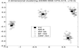
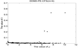
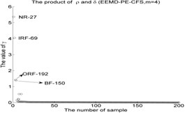
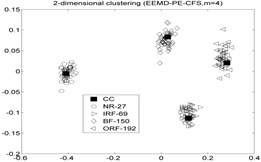
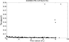
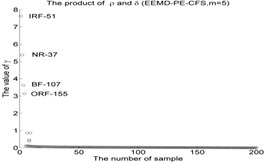
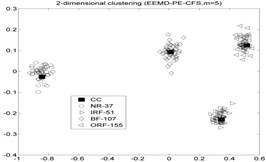
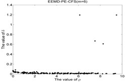
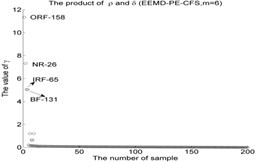
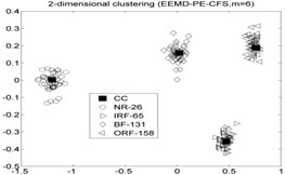
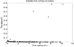
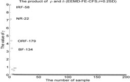
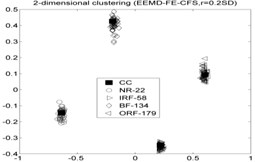
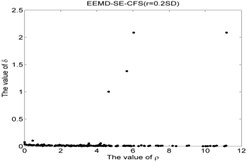
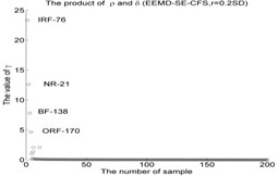
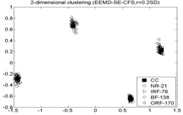
As shown in Fig. 4, the first two IMF-BSE/PE/FE/SE entropy values are higher than other IMF components. the first two IMF-BSE/PE/FE/SE values were selected as the input of CFS model according to the correlation values in Table 2, the results of local density ρ and distance δ of the clustering centers are given in Table 5, the figure of local density ρ, distance δ and 2-dimension clustering are shown in Fig. 5.
Table 5The value of local density ρ, distance δ and γ
Mode | The center point of each cluster | ρ | δ | γ |
EEMD-BSE-CFS (m=4, a= 0.2) | NR-13 | 11.8807 | 0.5676 | 6.7438 |
IRF-97 | 7.7101 | 0.5676 | 4.3764 | |
BF-128 | 9.2967 | 0.5055 | 4.6999 | |
ORF-177 | 4.4287 | 0.2552 | 1.1300 | |
EEMD-BSE-CFS (m= 4, a=0.3) | NR-47 | 11.2333 | 0.6432 | 7.2250 |
IRF-68 | 7.0638 | 0.6432 | 4.5432 | |
BF-139 | 9.4863 | 0.5743 | 5.4482 | |
ORF-158 | 4.5359 | 0.3031 | 1.3750 | |
EEMD-BSE-CFS (m= 5, a=0.2) | NR-48 | 10.8704 | 0.7167 | 7.7904 |
IRF-79 | 6.4877 | 0.1337 | 0.8671 | |
BF-136 | 4.5636 | 0.2610 | 1.1909 | |
ORF-172 | 6.8259 | 0.7167 | 4.8919 | |
EEMD-BSE-CFS (m= 5, a=0.3) | NR-6 | 10.7528 | 1.9290 | 20.7417 |
IRF-95 | 7.5217 | 1.9290 | 14.5091 | |
BF-150 | 6.6052 | 0.9898 | 6.5379 | |
ORF-161 | 5.3497 | 0.5566 | 2.9775 | |
EEMD-PE-CFS (m=4) | NR-27 | 10.0901 | 0.5317 | 5.3648 |
IRF-69 | 7.6169 | 0.5317 | 4.0498 | |
BF-150 | 6.4482 | 0.2152 | 1.3878 | |
ORF-192 | 6.9443 | 0.2044 | 1.4197 | |
EEMD-PE-CFS (m=5) | NR-37 | 6.2524 | 0.8601 | 5.3776 |
IRF-51 | 8.8701 | 0.8601 | 7.6290 | |
BF-107 | 7.9180 | 0.4578 | 3.6250 | |
ORF-155 | 8.0028 | 0.3918 | 3.1354 | |
EEMD-PE-CFS (m=6) | NR-26 | 6.1153 | 1.1961 | 7.3145 |
IRF-65 | 8.2617 | 0.6117 | 5.0536 | |
BF-131 | 7.5113 | 0.6695 | 5.0291 | |
ORF-158 | 9.4830 | 1.1961 | 11.3426 | |
EEMD-FE-CFS (r=0.2SD) | NR-22 | 8.1721 | 0.8737 | 7.1402 |
IRF-58 | 10.2425 | 0.8737 | 8.9491 | |
BF-134 | 4.7898 | 0.7107 | 3.4043 | |
ORF-179 | 7.5670 | 0.5790 | 4.3814 | |
EEMD-SE-CFS (r=0.2SD) | NR-21 | 6.0385 | 2.0876 | 12.6060 |
IRF-76 | 11.1762 | 2.0876 | 23.3315 | |
BF-138 | 2.6576 | 1.3806 | 7.8107 | |
ORF-170 | 4.6496 | 1.0023 | 4.6605 |
As shown in Table 5 and Fig 5, the symbol ‘CC’ denotes the clustering centers of each cluster. The meaning of “NR-13”in Fig. 5(3) is that the number of clustering center is 13 in NR signal. It can be seen from Fig. 5(1), Fig. 5(4), Fig. 5(7), Fig. 5(10), Fig. 5(13), Fig. 5(16), Fig. 5(19), Fig. 5(22) and Fig. 5(25) that the value of local density ρ and distance δ for the four outlier points are higher than other normal points obviously, but it simply means that these outlier points may become cluster centers, the product of local density ρ and distance δ are shown in Fig. 5(2), Fig. 5(5), Fig. 5(8), Fig. 5(11), Fig. 5(14), Fig. 5(17), Fig. 5(20), Fig. 5(23) and Fig. 5(26), it shows that the γ value of four outlier points are higher than other points, such as the 13th point in NR signal, choosing the clustering centers according to the value of γ in Eq. (12). In [28], the authors suggests that these outlier clustering centers have character of hop in all points such as the 13th point jump to 128th point in Fig. 5.2, the 177th point jump to normal points. The normal points not like the clustering centers, they have character of smooth in Fig. 5(2). The classification accuracy rate under different models are given in Table 6.
Table 6The classification accuracy rate under different models
Mode | The correct number of each cluster | Accuracy (%) | Total accuracy (%) | ||||||
NR | IRF | BF | ORF | NR | IRF | BF | ORF | ||
EEMD-BSE-CFS (m=4, a= 0.2) | 50 | 50 | 50 | 50 | 100 % | 100 % | 100 % | 100 % | 100 % |
EEMD-BSE-CFS (m=4, a= 0.3) | 50 | 50 | 50 | 50 | 100 % | 100 % | 100 % | 100 % | 100 % |
EEMD-BSE-CFS (m= 5, a= 0.2) | 50 | 50 | 50 | 49 | 100 % | 100 % | 100 % | 98 % | 99.5 % |
EEMD-BSE-CFS (m= 5, a= 0.3) | 50 | 50 | 50 | 50 | 100 % | 100 % | 100 % | 100 % | 100 % |
EEMD-PE-CFS (m=4) | 50 | 50 | 50 | 50 | 100 % | 100 % | 100 % | 100 % | 100 % |
EEMD-PE-CFS (m=5) | 50 | 50 | 50 | 50 | 100 % | 100 % | 100 % | 100 % | 100 % |
EEMD-PE-CFS (m=6) | 50 | 50 | 50 | 49 | 100 % | 100 % | 100 % | 98 % | 99.5 % |
EEMD-FE-CFS (r=0.2SD) | 50 | 50 | 50 | 50 | 100 % | 100 % | 100 % | 100 % | 100 % |
EEMD-SE-CFS (r=0.2SD) | 50 | 50 | 50 | 50 | 100 % | 100 % | 100 % | 100 % | 100 % |
As shown in Table 6 the highest accuracy is up to 100 %, which indicates that the CFS clustering algorithm performs well in solving fault recognition problem. The original signals are decomposed into a series of IMFs, but the first two IMFs are the highest frequency portion of the original signals [31], and other IMFs in descending order, therefore, the first two IMFs contains the main information of the original signals. The results of IMF-BSE/PE/FE/SE values are given in Fig. 4. It can be seen that IMF-BSE/PE/FE/SE entropy values are in descending order, at the same the time, the correlation degree between overall IMFs and the original signals are measured by using the correlation coefficient, Table 2 shows that the correlation values are in descending order. In order to make the data visualization and reduce information redundancy, hence the first two IMF-BSE/PE/FE/SE values are used as the input of the CFS clustering model. Because the irregularity of NR vibration signal is higher than the other three kinds of signals, compared with the NR signal, fault signals have vibration regularity, especially the IRF and ORF signals. But the regularity and self-similarity of BF signal is weaker than the IRF and ORF. Thus the irregularity of BF signal is the highest in three fault signals, therefore, the first two IMF-BSE/PE/FE/SE values are different in Fig. 4.
CFS clustering algorithm uses the value of local density ρ and distance δ between two points to determine the clustering centers. In [28], the larger value of γ for the ith sample point, the more possibility of the ith sample point become the cluster center point, the value of γ for cluster center point has obvious characteristic of jump when the cluster centers into non-cluster center, such as Fig. 5(2), Fig. 5(5), Fig. 5(8), Fig. 5(11), Fig. 5(14), Fig. 5(17), Fig. 5(20), Fig. 5(23) and Fig. 5(26). The entropy values of the same signal samples were similar, and the entropy values of the different signal samples are not the same, therefore, the value of γ for each center point has better discriminative. The CFS algorithm has its basis in the assumptions that cluster centers are surrounded by neighbors with lower local density ρ and that they are at a relatively large distance δ from any points with a higher local density ρ. After the cluster centers have been found, each remaining point is assigned to the same cluster as its nearest neighbor of higher density. So the fault recognition accuracy rate of CFS clustering algorithm is good.
As mentioned above. The fault diameters of and motor speed of roller bearings in Table. 1 are 01778 mm and 1750 rpm, then using the experiment data with 0.5334 mm and 1797 rpm to fulfill the fault recognition by EEMD-BSE/PE/FE/SE-CFS models. The classification accuracy rate under different models are given in Table 7, and the 2-dimension clustering are shown in Fig. 6. The symbol ‘CC’ denotes the clustering center points, the symbol “NR-29” denotes the 29th sample point which is regarded as the NR cluster center point in first sub-figure included in Fig. 6 (the corresponding serial number of sample are as follow: NR: 1-50, IRF: 51-100, BF: 101-150, ORF: 151-200). As shown in Table 7, the highest accuracy is also up to 100 %.
Fig. 6The 2-dimension clustering for all samples by using CFS model
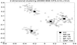
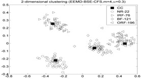
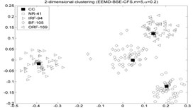
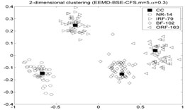
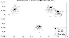
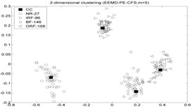
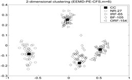
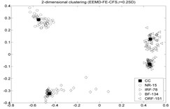
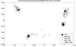
Table 7The classification accuracy rate under different models
Mode | The correct number of each cluster | Accuracy (%) | Total Accuracy (%) | ||||||
NR | IRF | BF | ORF | NR | IRF | BF | ORF | ||
EEMD-BSE-CFS (m=4, a=0.2) | 50 | 50 | 50 | 50 | 100 % | 100 % | 100 % | 100 % | 100 % |
EEMD-BSE-CFS (m=4, a=0.3) | 50 | 50 | 50 | 50 | 100 % | 100 % | 100 % | 100 % | 100 % |
EEMD-BSE-CFS (m=5, a=0.2) | 50 | 50 | 50 | 48 | 100 % | 100 % | 100 % | 96 % | 99 % |
EEMD-BSE-CFS (m=5, a=0.3) | 50 | 50 | 50 | 50 | 100 % | 100 % | 100 % | 100 % | 100 % |
EEMD-PE-CFS (m=4) | 50 | 50 | 50 | 48 | 100 % | 100 % | 100 % | 96 % | 99 % |
EEMD-PE-CFS (m=5) | 50 | 50 | 50 | 49 | 100 % | 100 % | 100 % | 98 % | 99.5 % |
EEMD-PE-CFS (m=6) | 50 | 50 | 50 | 49 | 100 % | 100 % | 100 % | 98 % | 99.5 % |
EEMD-FE-CFS (r=0.2SD) | 50 | 50 | 50 | 50 | 100 % | 100 % | 100 % | 100 % | 100 % |
EEMD-SE-CFS (r=0.2SD) | 50 | 50 | 50 | 50 | 100 % | 100 % | 100 % | 100 % | 100 % |
The classification accuracy rate by using EEMD-BSE-FCM/GK/GG models are given in Table 8, and the 2-dimension clustering are shown in Fig. 7.
It can be seen that the best total accuracy (%) is up to 100 % in Table 8, it is same as the 100 % by using EEMD-BSE/PE/SE/FE-CFS models, but the CFS algorithm which did not require pre-set the number of clustering centers, the cluster centers are characterized by a higher density than their neighbors and by a relatively large distance from points with higher densities. But the FCM/GK/GG model requires to pre-set the number of clustering centers
Fig. 7The 2-dimension clustering for all samples by using FCM/GK/GG clustering models
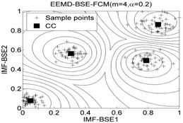
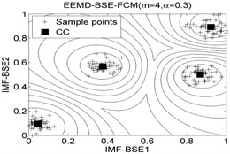
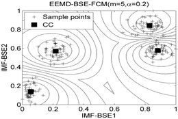
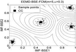
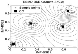
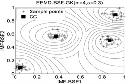
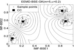
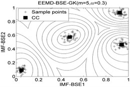
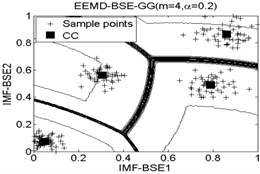
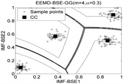
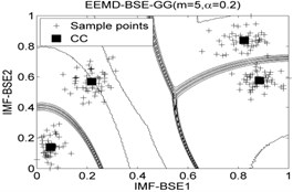
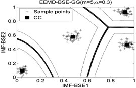
Table 8The classification accuracy rate under different models
Mode | The correct number of each cluster | Accuracy (%) | Total accuracy (%) | ||||||
NR | IRF | BF | ORF | NR | IRF | BF | ORF | ||
EEMD-BSE-FCM (m=4, a=0.2) | 50 | 50 | 50 | 50 | 100 % | 100 % | 100 % | 100 % | 100 % |
EEMD-BSE-FCM (m=4, a=0.3) | 50 | 50 | 50 | 50 | 100 % | 100 % | 100 % | 100 % | 100 % |
EEMD-BSE-FCM (m=5, a=0.2) | 50 | 50 | 50 | 48 | 100 % | 100 % | 100 % | 96 % | 99 % |
EEMD-BSE-FCM (m=5, a=0.3) | 50 | 50 | 50 | 50 | 100 % | 100 % | 100 % | 100 % | 100 % |
EEMD-BSE-GK (m=4, a=0.2) | 50 | 50 | 50 | 50 | 100 % | 100 % | 100 % | 100 % | 100 % |
EEMD-BSE-GK (m=4, a=0.3) | 50 | 50 | 50 | 50 | 100 % | 100 % | 100 % | 100 % | 100 % |
EEMD-BSE-GK (m=5, a=0.2) | 50 | 50 | 50 | 50 | 100 % | 100 % | 100 % | 100 % | 100 % |
EEMD-BSE-GK (m=5, a=0.3) | 50 | 50 | 50 | 50 | 100 % | 100 % | 100 % | 100 % | 100 % |
EEMD-BSE-GG (m=4, a= 0.2) | 50 | 50 | 50 | 48 | 100 % | 100 % | 100 % | 96 % | 99. % |
EEMD-BSE-GG (m=4, a=0.3) | 50 | 50 | 50 | 49 | 100 % | 100 % | 100 % | 98 % | 99.5 % |
EEMD-BSE-GG (m=5, a=0.2) | 50 | 50 | 50 | 49 | 100 % | 100 % | 100 % | 98 % | 99.5 % |
EEMD-BSE-GG (m=5, a=0.3) | 50 | 50 | 50 | 50 | 100 % | 100 % | 100 % | 100 % | 100 % |
6. Conclusions
A method based on EEMD, BSE and CFS for roller bearings is presented in this paper, the roller bearings vibration signals are decomposed into several IMFs, the correlation coefficient method was is to verify the correlation degree of IMFs and the corresponding original signal. The first two IMFs according to the value of correlation coefficient, the BSE/PE/FE/SE methods is used to calculate the IMF-BSE/PE/FE/SE values. Different from the PE/FE/SE methods, the BSE method make only use of the all adjacent points for calculating the BS value and construct the original signals once time, the results of elapsed time show that the computational efficiency of BSE method is faster than that of PE/FE/SE models. The first two IMF-BSE/PE/FE/SE are regarded as the input of CFS clustering algorithm, the CFS clustering algorithm which did not require pre-set the number of clustering centers, it was determined by its local density and cutoff distance. Finally, the experiment results show that the computational efficiency of BSE model is faster than PE/FE/SE models under the same fault recognition accuracy rate.
References
-
Žvokelj M., Zupan S., Prebil I. Non-linear multivariate and multiscale monitoring and signal denoising strategy using kernel principal component analysis combined with ensemble empirical mode decomposition method. Mechanical Systems and Signal Processing, Vol. 25, 2011, p. 2631-2653.
-
William P. E., Hoffman M. W. Identification of bearing faults using time domain zero-crossings. Mechanical Systems and Signal Processing, Vol. 25, 2011, p. 3078-3088.
-
Yuan S. F., Chu F. L. Fault diagnostics based on particle swarm optimization and support vector machines. Mechanical Systems and Signal Processing, Vol. 21, 2007, p. 1787-1798.
-
Lei Y., He Z., Zi Y. EEMD method and WNN for fault diagnosis of locomotive roller bearings. Expert Systems with Applications, Vol. 38, 2011, p. 7334-7341.
-
Pincus S. M. Approximate entropy as a measure of system complexity. Proceedings of the National Academy of Sciences, Vol. 88, 1991, p. 2297-2301.
-
Yan R. Q., Gao R. X. Approximate entropy as a diagnostic tool for machine health monitoring. Mechanical Systems and Signal Processing, Vol. 21, 2007, p. 824-839.
-
Richman J. S., Moorman J. R. Physiological time-series analysis using approximate entropy and sample entropy. American Journal of Physiology – Heart Circulatory Physiology, Vol. 278, Issue 6, 2000, p. 2039-2049.
-
Zhu K. H., Song X. G., Xue D. X. Fault diagnosis of rolling bearings based on IMF envelope sample entropy and support vector machine. Journal of Information and Computational Science, Vol. 10, Issue 16, 2013, p. 5189-5198.
-
Chen W. T., Zhuang J., Yu W. X., et al. Measuring complexity using FuzzyEn, ApEn, and SampEn. Medical Engineering and Physics, Vol. 31, 2009, p. 61-68.
-
Chen W. T., Wang Z. Z., Xie H. B., et al. Characterization of surface EMG signal based on FuzzyEntropy. IEEE Transactions on Neural Systems and Rehabilitation Engineering, Vol. 15, Issue 2, 2007, p. 266-272.
-
Zheng J. D., Cheng J. S., Yang Y. A rolling bearing fault diagnosis approach based on LCD and fuzzy entropy. Mechanism and Machine Theory, Vol. 70, 2013, p. 441-453.
-
Bandt C., Pompe B. Permutation entropy: a natural complexity measure for time series. Physical Review Letters, Vol. 88, 2002, p. 174102.
-
Zhang X. Y., Liang Y. T., Zang Y., et al. A novel bearing fault diagnosis model integrated permutation entropy, ensemble empirical mode decomposition and optimized SVM. Measurement, Vol. 69, 2015, p. 164-179.
-
Yan R. Q., Liu Y. B., Gao R. X. Permutation entropy: a nonlinear statistical measure for status characterization of rotary machines. Mechanical Systems and Signal Processing, Vol. 29, 2012, p. 474-484.
-
Tiwari R., Gupta V. K., Kankar P. K. Bearing fault diagnosis based on multi-scale permutation entropy and adaptive neuro fuzzy classifier. Journal of Vibration and Control, 2013, p. 1-7.
-
Li J., Ning X. B. Dynamical complexity detection in short-term physiological series using base-scale entropy. Physical Review E, Vol. 73, 2006, p. 052902.
-
Liu D. Z., Wang J., Li J., et al. Analysis on power spectrum and base-scale entropy for heart rate variability signals modulated by reversed sleep state. Acta Physica Sinica, Vol. 63, 2014, p. 198703.
-
Rafiee J., Rafiee M. A., Tse P. W. Application of mother wavelet functions for automatic gear and bearing fault diagnosis. Expert Systems with Applications, Vol. 37, 2010, p. 4568-4579.
-
Lou X. S., Loparo A. Kenneth Bearing fault diagnosis based on wavelet transform and fuzzy inference. Mechanical Systems and Signal Processing, Vol. 18, 2004, p. 1077-1095.
-
Huang N. E., Shen Z., Long S. R., et al. The empirical mode decomposition and the Hilbert spectrum for nonlinear and non-stationary time series analysis. Proceedings of The Royal Society a Mathematical Physical and Engineering Sciences, Vol. 454, 1998, p. 903-995.
-
Wu H. Z., Huang N. E. Ensemble empirical mode decomposition: a noise-assisted data analysis method. Advances in Adaptive Data Analysis, Vol. 1, 2009, p. 1-41.
-
Zhang X. Y., Zhou J. Z. Multi-fault diagnosis for rolling element bearings based on ensemble empirical mode decomposition and optimized support vector machines. Mechanical Systems and Signal Processing, Vol. 41, 2013, p. 127-140.
-
Tang R. L., Wu Z., Fang Y. J. Maximum power point tracking of large-scale photovoltaic array. Solar Energy, Vol. 134, 2016, p. 503-514.
-
Gu B., Sheng V. S. A robust regularization path algorithm for v-support vector classification. IEEE Transactions on Neural Networks and Learning Systems, 2016, p. 1-8.
-
Zheng Y. H., Jeon B., Xu D. H., et al. Image segmentation by generalized hierarchical fuzzy C-means algorithm. Journal of Intelligent and Fuzzy Systems, Vol. 28, Issue 2, 2015, p. 124-144.
-
Zhang S. Q., Sun G. X., Li L., et al. Study on mechanical fault diagnosis method based on LMD approximate entropy and fuzzy C-means clustering. Chinese Journal of Scientific Instrument, Vol. 34, Issue 3, 2013, p. 714-720.
-
Gustafson D. E., Kessel W. C. Fuzzy clustering with fuzzy covariance matrix. IEEE Conference on Decision and Control including the 17th Symposium on Adaptive Processes, 1979, p. 761-766.
-
Wang S. T., Li L., Zhang S. Q., et al. Mechanical fault diagnosis method based on EEMD sample entropy and GK fuzzy clustering. Chinese Journal of Scientific Instrument, Vol. 24, Issue 22, 2013, p. 3036-3044.
-
Gath I., Geva A. B. Unsupervised optimal fuzzy clustering. IEEE Transactions on Pattern Analysis and Machine Intelligence, Vol. 11, Issue 7, 1989, p. 773-781.
-
Bezdek J. C., Dunn J. C. Optimal fuzzy partitions: a heuristic forb estimating the parameters in a mixture of normal distributions. IEEE Transactions on Computers, 1975, p. 835-838.
-
Rodriguez A., Laio A. Clustering by fast search and find of density peaks. Science, Vol. 344, Issue 3191, 2014, p. 1492-1496.
-
The Case Western Reserve University Bearing Data Center Website Bearing data center test seeded fault test data. http://csegroups.case.edu/bearingdatacenter/pages/download-data-file, 2013.
-
Zheng J. D., Cheng J. S., Yang Y., et al. A rolling bearing fault diagnosis method based on multi-scale fuzzy entropy and variable predictive model-based class discrimination. Mechanism and Machine Theory, Vol. 78, 2014, p. 187-200.
Cited by
About this article
This work was supported by the National Natural Science Foundation of China (Grant No. 61201168).
Fan Xu and Yan Jun Fang contributed to the conception of the study. Rong Zhang helped perform the analysis with constructive discussions. Xin Li and Zheng Min Kong contributed significantly to analysis and manuscript preparation.
