Abstract
In this paper, a data driven method based on Ensemble Empirical Mode Decomposition-Principal Component Analysis (EEMD-PCA) and Least Square-Support Vector Machine (LS-SVM) is proposed to achieve residual useful life (RUL) prediction for slewing bearings. Firstly, life-cycle vibration signals are acquired and divided into several signal segments, and EEMD is then utilized to decompose each segment into Intrinsic Mode Functions (IMFs). Afterwards, PCA is introduced to illustrate the trends of each IMF across the life cycle, and some of the IMFs that contribute to reveal the performance degradation process of the slewing bearing are selected to reconstruct and de-noise the vibration signals. After that, continuous squared prediction error (C-SPE) and its features are presented as performance degradation indicators. Finally, an RUL prediction model is built on the basis of the indicators using LS-SVM. The results of a life-cycle experiment show that the C-SPE of the de-noised vibration signals can precisely explain the performance degradation process of the tested slewing bearing and that the established RUL prediction model is close to practice. Besides, a comparison study shows that the C-SPE based RUL prediction model is more efficient and accurate than the signal based model. Therefore, the proposed method ensures high-reliability slewing bearing prognostics.
1. Introduction
Slewing bearings are important rolling rotational connections in many large-size machineries. The complete failure of a slewing bearing may bring disastrous loss to an enterprise, and even cause significant social impacts. Accurate RUL prediction may help enterprises to make timely maintenance or replacement schedules, which can effectively avoid catastrophic incidents. In recent years, with the development of sensor technology, more and more researchers have expressed their interest in data driven based RUL prediction. In most cases, an RUL prediction model should include three steps: signal de-noising, performance degradation features extraction and RUL prediction modeling.
EEMD has been widely used in current de-noising and feature extraction methods. Jiang et al. [1] combined EEMD and self-zero space projection analysis to identify faults in rotor-bearing systems, and successfully applied the method to bearing vibration signals. Similarly, Ahn et al. [2] developed a bearing fault detection method by using a wavelet de-nosing scheme and proper orthogonal value (POV) of the first IMFs covariance matrix. Experimental results demonstrated the feasibility of wavelet-based de-noising and exhibited that the POV provides more reliable fault detection results in some cases. Besides, Zvokelj et al. [3, 4] presented an EEMD-MSPCA based de-noising and diagnosing approach for slewing bearings, and contrastive study showed that their proposed method can achieve a better de-noising result compared with wavelet de-noising. However, two empirical parameters in their de-noising procedure are difficult to be obtained in practice. Moreover, Widodo et al. [5] utilized multi-class relevance vector machine (RVM) and SVM to detect an incipient fault of low speed bearings. Savitzky-Golay filtering and self-organizing map were employed to achieve de-noising and bearing health assessment respectively in literature [6, 7]. Caesarendra et al [8] conducted a slewing bearing life test, and fault frequency was successfully extracted by EEMD and FFT. In addition, they [9] introduced four circular-domain features to identify the slight changes of bearing condition, and the proposed method was proved better than time-domain methods in condition monitoring. However, they also pointed out that the circular-domain features are unable to assess the failure degradation trend. In terms of RUL prediction, SVM and its relative methods, such as support vector regression (SVR), support vector data descriptions (SVDD) and LS-SVM are most commonly used methods. Dong et al. [10, 11] firstly calculated time-domain, frequency-domain and time-frequency-domain features, and then proposed a novel method combines PCA with LS-SVM to predict bearing degradation trend. A data mining approach using machine learning technique called anomaly detection (AD) was presented in literature [12]. The method employed kurtosis and Non-Gaussianity Score (NGS) to develop anomaly detection algorithms, which was proved sensitive and accurate to early stage anomalies. Tran et al. [13] provided a three-stage method for assessing the machine health degradation and forecasting the RUL. Firstly, an identification model was built on normal signals, and then RMS of residual errors was considered as the degradation indicator and survival function was established based on Cox’s proportional hazard model. Finally, SVM and time series techniques were used to forecast the RUL.
It can be seen from the above that methods for vibration signal de-noising and feature extraction have been deeply studied in recent years, and wavelet, EEMD and PCA are among the most commonly used methods. Besides, as a reliable machine learning technique, SVM is suitable for equipment degradation trend forecasting. However, the periodical impact in naturally damaged slewing bearing vibration signals is usually very weak because of the large size and low speed of slewing bearing, which makes the vibration signals almost completely overwhelmed by white noise. As a result, the first few IMFs usually contain a large amount of noise, and this may lead to improper selection of these IMFs by current methods [2, 8, 10, 11]. Besides, unlike those purposely manufactured defects [2-4, 10], possible faults of a slewing bearing raceway are usually indentation, pitting, cracking and spalling, which may result in even weaker impulse components in vibration signals. Moreover, current feature extraction methods mostly focus on fault frequency extraction while the frequency itself cannot be a proper performance degradation indicator. In addition, multi-dimensional vibration signals can better describe a slewing bearing condition than one dimensional signal [3, 4], whereas current life prediction methods [10, 11] may bring dimension disasters if applied to multi-dimensional cases. Therefore, commonly used signal processing methods cannot be directly applied to slewing bearing vibration signals, which brings a lot of challenges for slewing bearing diagnostics and prognostics.
To address the challenges mentioned above, this paper presents a novel method for slewing bearing RUL prediction. First of all, an EEMD-PCA based method is proposed to achieve de-noising by selecting the most representative components in vibration signals, which focuses on life-cycle vibration signals instead of a short period of signal. Secondly, C-SPE and its features are introduced to indicate the trends of multi-dimensional vibration signals, namely, the performance degradation trend of a slewing bearing. Last but not least, LS-SVM is utilized to predict the RUL by establishing the relationship between extracted features and RUL. The rest of this paper is organized as follows: Section 2 contains the theoretical background of EEMD, PCA and LS-SVM methods. As detailed descriptions of these methods can be found elsewhere, this paper only presents the general principles of these methods. In Section 3, the proposed method is explained in detail. The effectiveness of the proposed method for slewing bearing RUL prediction and the comparisons with some commonly used methods, along with a detailed description of the test rig and an integrated measuring system, are presented in Section 4. Finally, some concluding remarks are drawn in Section 5.
2. Background knowledge
2.1. Ensemble empirical mode decomposition
As a self-adaptive data-driven method, Empirical Mode Decomposition (EMD) is very suitable for unstable signal processing. However, the non-linear components in non-stationary signals may result in different frequency scales projected on one IMF, and this phenomenon is also called mode mixing. To solve this problem, Wu and Huang [14] proposed the Ensemble Empirical Mode Decomposition method in 2009, which put white noise in EMD procedures to restrain mode mixing effect. For signal a(t), the procedures of EEMD are as follows:
(I) Put a randomly generated white noise s(t) with magnitude z to raw signal a(t) to generate a new data set anew(t):
(II) Use EMD to decompose anew(t) into H IMFs, the h-th (h∈[1,H]) IMF is represented as fh(t).
(III) Repeat steps (I) and (II) I times with different white noise series to obtain an ensemble of IMFs, the hth (h∈[1,H]) IMF after ith (i≤I) EMD is fih(t).
(IV) Obtain the hth IMF of EEMD by calculating the ensemble means of corresponding IMFs:
It should be noted that, the magnitude of white noise z and the repeated times I need to be determined during EEMD process. Chen et al. [15] pointed out that under a same noise level, z is not a critical factor to calculation results, and the increase of I can only slow down the calculation. Therefore, in this paper, z is 0.2 and I is 100.
2.2. Principal component analysis
PCA de-correlates variables through extraction of linear relationships between variables, and uses several unrelated components to represent all variables. For matrix X(m×n), where m represents the number of samples and n stands for the number of variables, PCA decomposes it into principal component space and residual subspace:
where tj (m×1) is the jth principal component (PC), pj (n×1) stands for the jth load vector, and E represents the residual error. X can also be presented as:
where T(m×r) is the principal component matrix, and P(n×r) is the load matrix.
Therefore, the projection on residual space is:
To implement condition monitoring, most PCA based schemes use two typical statistical indices: Hotelling’s T2 and squared prediction error (SPE), also known as Q statistic. According to literature [16], SPE can better demonstrate the differences between new datasets and the original dataset. Meanwhile, it would be seen as abnormality if the overall trend of the vector SPE is greater than its threshold Qα, and they can be calculated by Eqs. (6), (7):
where is the standard normal deviate corresponding to the upper () percentile, for 1, 2, 3, , and is the th eigenvalue of the variance–covariance matrix of input data .
2.3. Least square – support vector machine
Proposed by Vapnik [17], SVM was developed to solve pattern recognition problems based on the structural risk minimization theory. With SVM, different data sets are firstly separated by hyperplanes as much as possible, and then an optimal hyperplane will be found to maximize the distances between all the hyperplanes. The normal vectors of the optimal hyperplane are called support vectors. In order to improve machine learning speed, LS-SVM [18] was then proposed to transfer a quadratic programming problem into a one-dimensional linear problem by replacing the insensitive loss function used in SVM with a squared error loss function.
For an sample training set {, }, 1, 2,…, , where () is the th input vector while () represents the output. The linear regression function of LS-SVM is:
where stands for the mapping function in kernel space, represents the normal vector of the hyperplane and is a constant. This linear problem can also be described as:
where is the training error, is defined as a regularization parameter to adjust the penalty for training errors. By introducing Lagrange multipliers and optimal constraints, the LS-SVM prediction model can be described as:
where is the kernel function, which maps the sample space into a high-dimensional space. It should be noted that commonly used kernel functions are linear kernel function, polynomial kernel function and radial basic function (RBF).
3. Methodology
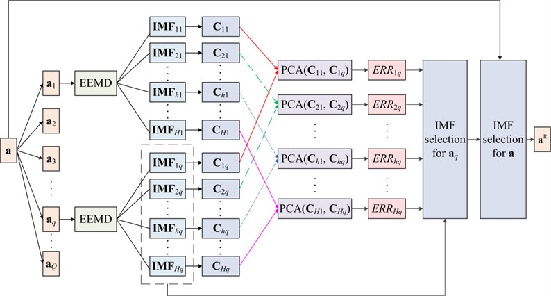
The flowchart of the proposed method is shown in Fig. 1, which contains four steps: raw data acquisition, signal de-noising, performance degradation features extraction and RUL prediction. First of all, groups of vibration signals are acquired by a slewing bearing life-cycle test. Secondly, all acquired signals are de-noised by the proposed de-noising method, which is shown in Fig. 2.
For a life-cycle vibration signal , the detailed de-noising steps are as follows:
(1) Divide into segments, and the th () segment is defined as .
(2) Decompose each segment into H IMFs using the EEMD method, and () stands for the th IMF of ().
(3) Split the into multi-dimensional matrix , and a PCA model is built based on .
(4) Split the into multi-dimensional matrix . Afterwards, is projected onto the PCA model built in step (3) and the statistics is calculated as . If is obviously greater than the threshold of the statistics, then it is supposed that there is some abnormality in the th IMF of compared with the th IMF of . To quantify this analysis, ERR is introduced to describe the difference between the th IMF of and the th IMF of , and is then obtained by using the mean of minus the threshold of the statistics. Given that is acquired under a healthy condition, the can also represent the abnormality in the th IMF of . It should be also noted that the sensitivity of each IMF to the performance degradation of equipment is different. Hence, for signal , the higher the more sensitive to abnormality the , and these sensitive IMFs will be selected to reconstruct .
(5) Define () as the weight factor, when the share of the sum of the () biggest ERRs in the sum of all ERRs is larger than , the corresponding IMFs are selected to reconstruct . Meanwhile, given the randomness of white noise, the first few IMFs which contain high frequency components (including white noise) change little at different time periods. Consequently, the ERRs of these IMFs are usually little, and these IMFs will be neglected during the selection procedure. By doing so, the reconstructed not only reserves the performance degradation features, but also achieves de-noising.
(6) However, different slewing bearing faults (such as ball crack, inner ring spalling and so forth) may result in different fault frequencies, which further leads to different IMF selections when ranges from 1 to . In order to select a certain group of IMFs to reconstruct life-cycle signal , all the selected IMFs mentioned above are sorted by their selected times, and a few most frequently selected IMFs will be utilized to reconstruct the life-cycle signal .
Fig. 1Flowchart of the proposed method

After de-noising, the th () segments of the groups of vibration signals are combined into a matrix :
Afterwards, another PCA model is established based on , and then , ,…, are projected onto the PCA model to obtain the statistics (), respectively. By connecting every (), C-SPE is then acquired to reveal the changes of the -dimensional vibration signals relative to the early-stage (normal) vibration signals. Finally, C-SPE and its time-domain features are introduced as the input, and the RUL of the slewing bearing is output, an LS-SVM based RUL prediction model can be established for slewing bearing prognostics.
It can be observed that our proposed method differs from commonly used signal processing methods in several aspects. To start with, most current methods focus on fault frequency extraction from signals with a time length of seconds or even less. However, as mentioned above, the weak impulse components in vibration signals generated by a slewing bearing are hard to extract, and the fault frequency itself is not a suitable indicator to reveal the performance degradation process of equipment. Instead, the proposed method focuses on life-cycle vibration signals, and achieves de-noising by selecting the most representative components in vibration signals. What’s more is that, the proposed method focuses on the performance degradation trends of equipment while not frequency extraction, which provides a potential for RUL prediction modeling. Besides, current methods [10, 11] may bring dimension disasters when processing multi-dimensional vibration signals, whereas the proposed method introduces C-SPE and its time-domain features to achieve both dimensionality reduction and potential performance degradation trends indication. It should be noted that all the characteristics of the proposed method mentioned above will be thoroughly validated in Section 4.
Fig. 2Procedure of the proposed de-noising method
4. Experimental validation
4.1. Experimental setup and results.
To evaluate the performance of the proposed method, a home-made test platform is developed to implement an experiment. As shown in Fig. 3, G1, G2 and G3 are hydraulic rams to apply axial force, radial force and turnover movement to a tested slewing bearing, and G4 is the hydraulic motor to drive the slewing bearing. More information of the test platform can be found in Table 1.
Fig. 3Home-made test platform
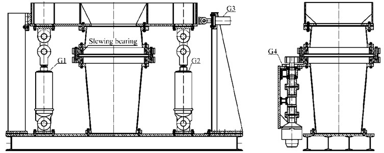
Table 1Capacity of the test platform
Size [m] | Power [kW] | Axial force [kN] | Radial force [kN] | Turnover moment [kN·m] | Rotational speed [r/min] | Diameter of the slewing bearing [mm] |
3.4×1.4×2.1 | 20 | 0-750 | 101.8 | 0-880 | 0.5-5 | 600-2000 |
As shown in Fig. 4 and Fig. 5, the type of the main tested slewing bearing is QNA-730-22, of which the inner ring is the rotatable ring and the outer ring is the fixed ring. The properties of the slewing bearing are shown in Table 2.
Table 2Properties of the main tested slewing bearing
Average diameter [mm] | Ball diameter [mm] | Extreme axial force [kN] | Extreme radial force [kN] | Extreme turnover moment [kN·m] | Extreme rotational speed [r/min] |
730 | 22 | 96 | 35 | 246 | 10 |
Fig. 4Improved test platform for validation of the proposed method
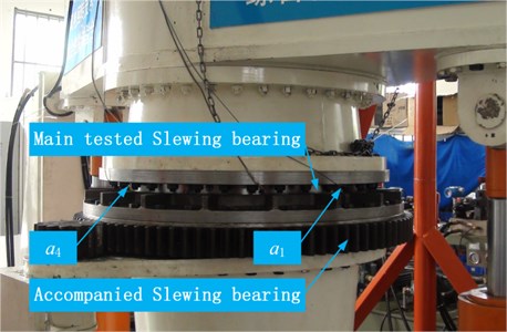
Given that the tested slewing bearing is inner geared, some improvements have been made to the test platform. With the frocks shown in Fig. 4, the inner ring (with gears) of the main tested slewing bearing is connected with the outer ring of the accompanied slewing bearing, and the outer (fixed) ring of the main tested slewing bearing is fixed with the upper flange. After which, as shown in Fig. 5, extreme loads are applied to the main tested slewing bearing and the experiment starts at a constant speed of 4 r/min.
Fig. 5Applied loads and the distribution of the four accelerometers
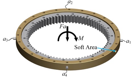
To implement condition monitoring, as shown in Fig. 5, four 495 mv/g Kistler-8395A010 accelerometers are mounted along the radial direction of the slewing bearing for vibration measurement, and the vibration signals are collected by NI PXIe-4492 at a sampling rate of 2 kHz. Besides, to assist monitoring the slewing bearing condition, the grease temperature, driven torque and rotational speed are also measured by NI PXI-6238 at a sampling rate of 10 Hz. What’s more, the main data acquisition (DAQ) system, NI PXIe-1062Q collects all the data from both PXIe-4492 and PXI-6238 through a LabVIEW interface. The schematic of the DAQ system is shown in Fig. 6.
Fig. 6DAQ system schematic diagram
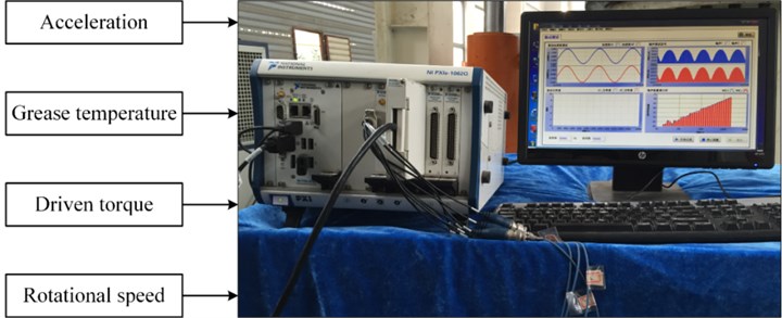
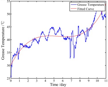
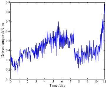
The test stops when the slewing bearing gets stuck and comes to a critical failure after 11 days, and the final amount of the turning laps of the slewing bearing is 6.33×10⁴. Fig. 7(a) and Fig. 7(b) show the trends of the grease temperature and the driven torque respectively. It should be specially explained that, to study the slewing bearing condition when its fatigue life reaches the Chinese standard [19] of 30000 r, we suspended the test and maintained the tested slewing bearing on the 7th day, and that’s the reason that both the grease temperature and the driven torque decrease after the 7th day. Besides, Fig. 7 also illustrates that both the grease temperature and the driven torque increase dramatically after the 9th day until the slewing bearing comes to a critical failure. In addition, Fig. 8(a) shows the slip zone occurred in the outer ring raceway of the tested slewing bearing on the 7th day, while Fig. 8(b) and Fig. 8(c) show the damaged outer ring and the cracked balls respectively when the slewing bearing gets stuck.
Fig. 7Trends of both the grease temperature and the driven torque during whole test: a) trend of the grease temperature and b) trend of the driven torque
a)
b)
4.2. RUL prediction and discussions
The lowest fault frequency of the tested slewing bearing is 0.34 Hz according to the commonly used bearing fault frequency calculation equations [20], and 0.34 Hz will have one full cycle period in at least 2.9 seconds [8]. Besides, during the whole test, vibration signals acquired at late night may reduce the environmental interferences as much as possible. Therefore, as shown in Fig. 9, we choose 3 seconds late-night acquired vibration data (6144 samples) of each day for signal processing and RUL prediction.
Fig. 8Damaged slewing bearing parts
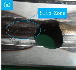
a) Slip zone
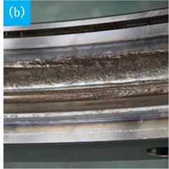
b) Damaged outer ring
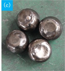
c) Cracked balls
Fig. 9Measured life-cycle vibration signals
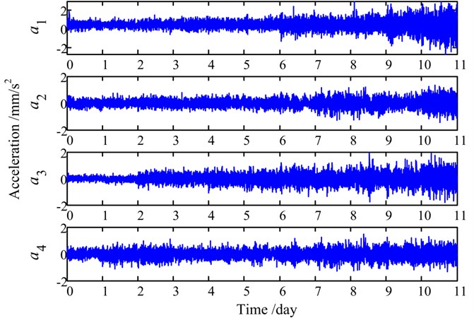
It can be observed from Fig. 9 that the details of all four signals are submerged under white noise and the energy of the periodical impulse is very low. For simplicity, only the de-noising procedures of will be presented below and the de-noising effectiveness will be compared with another EEMD-PCA based de-noising method [6]. Firstly, signal is divided into 11 segments according to the experimental days, and then all the signal segments are decomposed by EEMD respectively. The IMFs of the 5th signal segment are shown in Fig. 10 as an example.
Afterwards, the first IMF of both the 5th signal segment and the 1st signal segment are divided into matrix and respectively, and a PCA model is built on . Then, by projecting onto the PCA model, can be obtained. Accordingly, the ERRs of all 12 IMFs of the 5th signal segment are calculated.
By repeating the above steps, the ERRs of all 13 IMFs of the remaining signal segments can also be calculated. Fig. 11 visualizes the waterfall profile of the ERR amplitude vs. experimental days (signal segments) of all 13 IMFs, in which the red dot indicates that the curve is greater than zero for the first time. As mentioned above, the amplitude of the ERR represents the degree of abnormality in the corresponding IMF, while the abnormality of the IMF is the result of some fault occurred in the tested slewing bearing. Therefore, it can be observed from Fig. 11 that some incipient abnormalities occur in the 8th-12th IMFs from the 2nd day to the 4th day, which indicates the run-in period of the slewing bearing. Two days later, abnormalities firstly occur in the 5th-7th IMFs and keep being more severe, and the ERR amplitudes of the 8th-12th IMFs keep increasing at the same time. This phenomenon stands for the performance degradation process of the slewing bearing, and different types of slewing bearing faults are projected onto different IMFs. After the 9th day, the ERR amplitudes of the 6th-9th IMFs increase rapidly, which demonstrates the critical failure of the slewing bearing. It also should be noted that, in accordance with our previous statement, the ERR amplitudes of the first four IMFs keep low and change little throughout the experiment because of white noise, which will result in neglect of these IMFs in the selection process.
Fig. 10IMF 1-13 of the 5th signal segment of a1
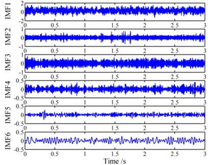
a) IMF 1-6 of the 5th signal segment
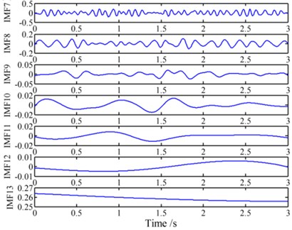
b) IMF 7-13 of the 5th signal segment
Fig. 11Trend of the ERR of each IMF in 11 days
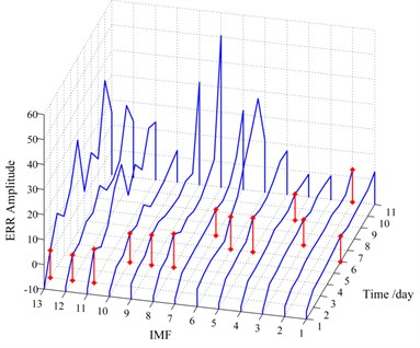
Fig. 12Profile of the ERR amplitude vs. all 13 IMFs of each day
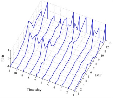
Table 3Selected IMFs for reconstructing the signal segment of each day
Day | 1 | 2 | 3 | 4 | 5 | 6 | 7 | 8 | 9 | 10 | 11 |
Selected IMFs | 6, 8, 11 | 11, 12 | 6, 11, 12 | 8, 11, 12 | 8-12 | 5, 6, 11, 12 | 5, 6, 11, 12 | 5, 6, 11, 12 | 5, 6, 8, 11, 12 | 5-8, 11, 12 | 8, 9, 11, 12 |
Nevertheless, Fig. 11 only exhibits the trends of the ERRs of each IMF throughout the experiment. It is still not clear enough for us to determine which IMFs to choose to reconstruct signal . Hence, take another look at Fig. 11, Fig. 12 demonstrates the waterfall profile of the ERR amplitude vs. all 13 IMFs of each day. It should be noted that the ERRs of each day are mapped to [–1, 1] respectively to clearly demonstrate which IMFs to be selected. For 0.9, the selected IMFs are listed in Table 3, and the selected times of each IMF are shown in Fig. 13.
Fig. 13Selected times of each IMF
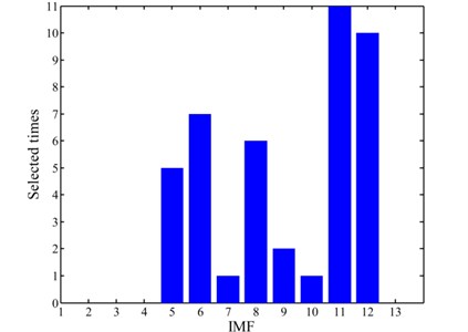
Therefore, the 5th, 6th, 8th, 11th and 12th IMFs are selected to reconstruct the life-cycle signal to achieve de-noising, and all the four groups of de-noised vibration signals are shown in Fig. 14.
Fig. 14De-noised life-cycle vibration signals by the proposed method
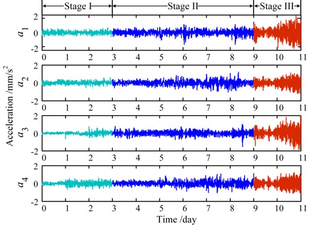
As shown in Fig. 14, the life-cycle signals are divided into three stages according to the trends of the vibration signals throughout the experiment. The amplitudes of the signals are low and stable at stage I, and then increase gradually at the middle stage. Before the end of the experiment, the amplitudes of signals rise dramatically and some periodical impulses can be found at stage III.
Meanwhile, for comparison, another EEMD-PCA based de-noising method [6] (we define it as direct EEMD-PCA) is utilized to de-noise the four groups of vibration signals. The de-noised signals and the contribution of each IMF (principal component) of are shown in Fig. 15(a) and Fig. 15(b) respectively. It can be seen from Fig. 15(b) that the contribution of the first five IMFs is very significant, and this will result in improper selection of the first few IMFs which contain large amount of white noise. Consequently, this method de-noises the raw signals to a certain extent, but the de-noised signals in Fig. 15(a) are still submerged by noise. Through the comparison, we can find out that, by selecting the most representative IMFs from life-cycle signals, the proposed de-noising method has a better de-noising effect on such low signal-to-noise vibration signals than direct EEMD-PCA based methods.
Fig. 15Direct EEMD-PCA de-noising
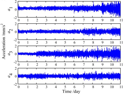
a) De-noised signals by direct EEMD-PCA
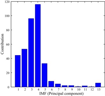
b) Contribution of each IMF (PC) of
After de-noising, two time-domain features: root mean square (RMS) values and impulse factors of the four groups of vibration signals are calculated and shown in Fig. 16(a) and Fig. 16(b) respectively. It can be seen from Fig. 16(a) that the overall trend of the RMS for each vibration signal is in accordance with a general performance degradation trend of equipment, while the details differences are caused by some random factors such as geometric errors, processes and loads. Fig. 16(b) illustrates the potential faults development in different positions of the slewing bearing. On one hand, since the accelerometer and are mounted near the load points, their peak values of the impulse factors are quite high, which indicates severe damages of the slewing bearing around sensor and . On the other hand, the peak values of the impact factor of appear more and earlier than , which demonstrates that the slewing bearing raceway around damages earlier and more severe because of the soft area. It is worthy to be found that all the phenomena observed from Fig. 16 are consistent with the conclusions drawn in our earlier work [21]. In a word, compared with one dimensional signal, multi-dimensional vibration signals can explain the performance degradation trend of the slewing bearing more thoroughly and precisely.
Fig. 16Two time-domain features
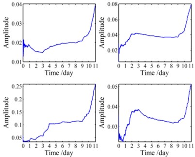
a) RMSs of the four de-noised signals
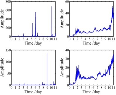
b) Impulse factors of the four de-noised signals
Nevertheless, the number of time-domain, frequency-domain and time-frequency-domain features of the four groups of vibration signals can reach up to 120 [10], which brings great challenges to RUL prediction modeling. To avoid dimension disasters, C-SPE of the four groups of signals and its RMS are calculated and shown in Fig. 17.
Fig. 17C-SPE and its RMS
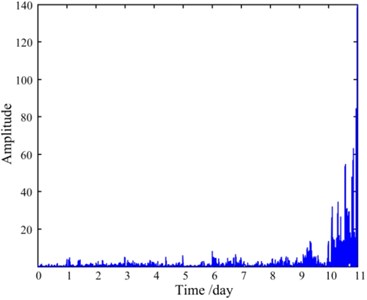
a) C-SPE of the four de-noised signals
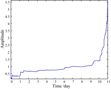
b) RMS of the C-SPE
It can be seen from Fig. 17 that the trend of the RMS of C-SPE is exactly in accordance with the performance degradation process of the slewing bearing observed above. The first three days reflect the run-in period, while the normal service period is demonstrated from the 3rd day to the 7th day. After maintenance, the condition of the slewing bearing improves a little on the 8th day, and soon after that, the condition becomes worse dramatically since the 9th day until a critical failure occurs. Therefore, C-SPE can be an effective feature to reduce the dimensions of the vibration signals and meanwhile accurately assess the performance degradation process as much as possible.
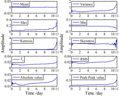
Given that the C-SPE in frequency domain has no practical significance, only ten dimensionless time-domain features of the C-SPE are calculated and shown in Fig. 18(a), which will be used as the inputs in RUL prediction modeling. At the same time, the same ten features of the four groups of de-noised signals are also calculated for comparison. For simplicity, only the features of are shown in Fig. 18(b).
Fig. 18Ten time-domain features of both C-SPE and a1
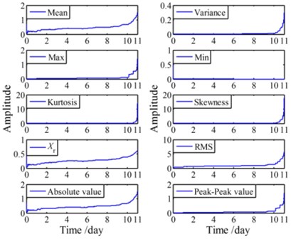
a) Features of C-SPE
b) Features of
Afterwards, to establish an RUL prediction model (C-SPE based model) with LS-SVM, ten time-domain features of the C-SPE and the residual useful life (expressed in revolutions) are introduced as the inputs and the outputs respectively. It should be noted that the kernel function used in the LS-SVM is the RBF, and the optimal regularization parameter and the kernel bandwidth in the RBF are determined by cross validation. In addition, another RUL prediction model (signal based model) is built based on the 40 time-domain features of the four groups of signals. Both of the established models are shown in Fig. 19.
Fig. 19LS-SVM based RUL prediction models
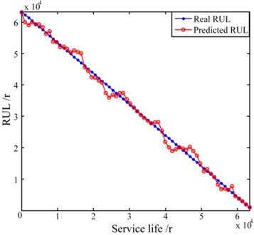
a) C-SPE based RUL prediction model: 103.22, 0.71, Time = 10.215 s, Accuracy = 99.40 %
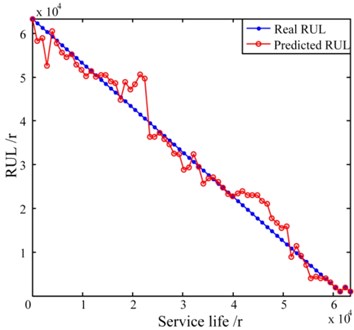
b) C-SPE based RUL prediction model: 75.14, 0.93, Time = 68.466 s, Accuracy = 94.30 %
It can be observed from Fig. 19 that the C-SPE based RUL prediction model has a shorter calculation time and a higher accuracy than the RUL prediction model built based on the features of signals. In fact, the C-SPE itself is an indication of the differences of signals in different time periods, therefore it can be seen from Fig. 17 and Fig. 18(a) that the C-SPE and most of its time-domain features keep increasing during the entire life cycle. On the contrary, as shown in Fig. 18(b), there are some fluctuations in many of the time-domain features of signals. Besides, the number of the input vectors of the C-SPE based model is only 10 while the number of the input vectors of the signal based model is up to 40. As a result, the signal based model is less accurate and more time consuming. It should be noted that the signal based model may achieve a higher performance if the input vectors are carefully selected from the 40 features. However, the selection procedure itself requires human involvement and thus is still inefficient.
5. Conclusions
In this paper, a data-driven based RUL prediction method for large-size low-speed slewing bearings is proposed, which consists of three steps: de-noising, performance degradation features extraction and RUL prediction modeling. An experimental validation is carried out and some interesting conclusions are drawn. Firstly, unlike conventional methods, the presented de-noising approach focuses on life-cycle vibration signals, and achieves a better de-noising effect by using EEMD-PCA to select the IMFs that are sensitive to abnormalities in signals. Secondly, multi-dimensional vibration signals can explain the performance degradation trend of the slewing bearing more sufficiently and thoroughly. Furthermore, instead of excessive features of multi-dimensional signals, the C-PSE and its ten time-domain features can also precisely assess the performance degradation process of the slewing bearing. Above all, the C-SPE based RUL prediction model is more efficient and accurate than the commonly used signal based RUL prediction model. Therefore, the proposed method may provide insight into the nature of equipment degradation in life-cycle vibration signals, and thus can be used as a reliable tool for large-size low-speed slewing bearings prognostics.
References
-
Fan J., Zhencai Z., Wei L., et al. Fault identification of rotor-bearing system based on ensemble empirical mode decomposition and self-zero space projection analysis. Journal of Sound and Vibration, Vol. 333, 2014, p. 3321-3331.
-
Jong-Hyo A., Dae-Ho K., Bong-Hwan K. Fault detection of a roller-bearing system through the EMD of a wavelet denoised signal. Sensors, Vol. 14, 2014, p. 15022-15038.
-
Matej Z., Samo Z., Ivan P. Non-linear multivariate and multiscale monitoring and signal denoising strategy using kernel principal component analysis combined with ensemble empirical mode decomposition method. Mechanical Systems and Signal Processing, Vol. 25, 2011, p. 2631-2653.
-
Matej Z., Samo Z., Ivan P. Multivariate and multiscale monitoring of large-size low-speed bearings using ensemble empirical mode decomposition method combined with principal component analysis. Mechanical Systems and Signal Processing, Vol. 24, 2010, p. 1049-1067.
-
Achmad W., Eric Y. K., Jong-Duk S.,et al. Fault diagnosis of low speed bearing based on relevance vector machine and support vector machine. Expert Systems with Applications, Vol. 36, 2009, p. 7252-7261.
-
Yu Z., Chris B., Zhijing Y. Machine fault detection by signal denoising – with application to industrial gas turbines. Measurement, Vol. 58, 2014, p. 230-240.
-
Jianbo Y. A hybrid feature selection scheme and self-organizing map model for machine health assessment. Applied Soft Computing, Vol. 11, Issue 5, 2011, p. 4041-4054.
-
Wahyu C., Prabuono Buyung K., Anh Kiet T., et al. Condition monitoring of naturally damaged slow speed slewing bearing based on ensemble empirical mode decomposition. Journal of Mechanical Science and Technology, Vol. 27, 2013, p. 2253-2262.
-
Wahyu C., Buyung K., Anh Kiet T., et al. Circular domain features based condition monitoring for low speed slewing bearing. Mechanical Systems and Signal Processing, Vol. 45, 2014, p. 114-138.
-
Shaojiang D., Tianhong L. Bearing degradation process prediction based on the PCA and optimized LS-SVM model. Measurement, Vol. 46, 2013, p. 3143-3152.
-
Shaojiang D., Shirong Y., Baoping T., et al. Bearing degradation process prediction based on the support vector machine and Markov model. Shock and Vibration, Vol. 2014, 2014, p. 1-15.
-
Afrooz P., Amir Hossein G., Mohammad E. A data mining approach for fault diagnosis: an application of anomaly detection algorithm. Measurement, Vol. 55, 2014, p. 343-352.
-
Van Tung T., Hong Thom P., Bo-Suk Y., et al. Machine performance degradation assessment and remaining useful life prediction using proportional hazard model and support vector machine. Mechanical Systems and Signal Processing, Vol. 32, 2012, p. 320-330.
-
Zhaohua W., Norden E. H. Ensemble empirical mode decomposition: a noise-assisted data analysis method. Advances in Adaptive Data Analysis, Vol. 1, 2009, p. 1-41.
-
Zhong C., Hechao F. Electromagnetic noise diagnosis for a permanent magnet synchronous motor based on EEMD. Journal of Vibration and Shock, Vol. 32, 2013, p. 124-128, (in Chinese).
-
Zhongjie S., Xuefeng C., Zhengjia H., et al. Remaining life predictions of rolling bearing based on relative features and multivariable support vector machine. Journal of Mechanical Engineering, Vol. 49, 2013, p. 183-189, (in Chinese).
-
Vladimir V. The Nature of Statistical Learning Theory. Springer, New York, 1995.
-
Suykens J., Gestel T., Brabanter J. Least Squares Support Vector Machines. World Scientific Publishers, Singapore, 2002.
-
Xiangshan X., Yuxia D., Fei L. Slewing Bearing. Chinese Patent No. JB/T2300-1999, 1999.
-
Shuting W., Luyong L., Yuling H. Fault diagnosis method of rolling bearing based on undecimated wavelet transformation of lifetime. Journal of Vibration and Shock, Vol. 28, 2009, p. 170-173, (in Chinese).
-
Yang F., Xiaodiao H., Jie C., et al. Reliability-based residual life prediction of large-size low-speed slewing bearings. Mechanism and Machine Theory, Vol. 81, 2014, p. 94-106.
About this article
The authors are grateful to the National Natural Science Foundation of China (Grant Nos. 51375222, 51175242).
