A bearing fault detection method with low-dimensional compressed measurements of vibration signal

1. Introduction

Considering the material defects, manufacturing errors, working conditions and other factors like fatigue, aging etc., the damages and faults of the rotating machinery occur inevitably during operation. The bearing is one of the most common and most important key components of the rotating machinery, in case of failure, this will lead to the equipment downtime which affects productivity and results in economic loss. Moreover, it might lead to accidents with extreme danger, which will threaten the safety of the entire equipment, even the staff. Thus, it is particularly important for rotating machinery to execute bearing condition monitoring and fault diagnosis.

The traditional monitoring method is achieved often by sampling the bearing vibration data under the Shannon sampling theorem. Then the bearing state information can be extracted from the vibration data, which is used in fault detection. The long-term and continuous monitoring needs to sample and store large amounts of raw vibration signal, which will burden the data storage and transmission greatly. The compressed sensing theory can provide a new idea in solving this problem. In 2006, Candès proved in mathematic principle that the original signal could be reconstructed using parts of its Fourier transform coefficients, which would be the theoretical foundation for compressed sensing [1]. Then Donoho and Candès et al proposed the concept of compressed sensing formally based on the related work [2, 3]. The main process of CS can be divided into two steps. First, combining the sampling with compressing, we can acquire the non-adaptive linear projections (or measurements) of the original signal. Then, the original signal can be reconstructed directly with these measurements by the appropriate recovery algorithms [4-7]. With this strategy, the amount of the data in monitoring will be reduced greatly and the burden in data transmission and storage will be alleviated effectively. Since it is possible to recover the original high-dimensional signal from the compressed measurements with low-dimension, which means that most of the bearing state information is contained in these low-dimensional measurements, then we can consider achieving the bearing fault detection just using the compressed measurements directly, without recovering the original signal. This is the starting point of our proposed method.

Some related researches based on the compressed sensing theory have been studied in the past several years. In reference [8-11], signal processing problems such as detection, classification, estimation and filtering problems are analyzed mathematically using only low-dimensional compressive measurements and without ever reconstructing the signals involved. In reference [12], the smashed filter for compressive classification and target recognition using very few measurements is proposed, which operated directly on the compressive measurements without first reconstructing the image. Reference [13] presents a technique for array diagnosis using a small number of measured data acquired by a near-field system by making use of the concepts of compressed sensing technique in image processing. In reference [14], the vibration data collected from the SHM system is used to analyze the data compression ability of compressed sensing. In reference [15], compressed sensing techniques is used to detect damage in structures, the compressed coefficients are collected from measurements, and then sending them to an off-board processor for signal reconstruction with over-complete dictionaries. The presence of damage is detected while using a relatively small number of compressed coefficients. In reference [16], a framework for the detection of stochastic signals from optimized projections in a noisy environment is proposed based on compressed sensing theory, dimensionality reduction techniques and support vector machines, which has higher accuracy and lower complexity than a scheme performing signal reconstruction first, followed by detection based on the reconstructed signal. Reference [17] proposes a damage identification scheme based on sparse representation of time domain structural responses and compressed sensing techniques, which can identify multiple types of damages, damage locations and severities even under high noise levels with minimum numbers of vibration measurements. Reference [18] proposed a parallel FISTA-like proximal decomposition algorithm for reconstruction of sparse time-frequency representation from the limited noisy observations based on compressed sensing theory, which is verified by detecting bearings and gears defects in rotating machines. The ability of compressed sensing in data compression was used in remote and offline condition monitoring of rotating machines. In reference [19], the compressed sensing technique is used in remote data transmission and introduced to compressing the data in ship side, and then the compressed data is transmitted to the shore side, in which the compressed data is decompressed. Combustion fault detection is achieved by time-frequency spectrum analysis based on the decompressed instantaneous angular speed data of marine diesel engines. In reference [20], the compressed sensing theory is introduced in fault diagnosis of train rolling bearing. The compressed sensing is used to compress the original signal, and the fault diagnosis process is achieved based on the recovered signal from the compressed signal.

The previous work which introduces compressed sensing in signal processing and fault diagnosis is mainly focus on two directions: one of them is the signal compression, and the main contribution of compressed sensing in these works is signal compression. The fault diagnosis is achieved based on the classical method with the reconstructed signal, which means that the original signal must be recovered first before fault diagnosing. Another direction is using the compressed signal directly in signal processing and fault diagnosis, without recovering the original signal. Most of these works are model-driven, which means that the information of the historical signals will not be used in these models.

In our paper, we introduced compressed sensing theory in bearing fault detection, which can be achieved using the compressed low-dimensional signal directly, without recovering the original signal first. The dictionary learning method is introduced in training the over-complete dictionary. Therefore, the historical data is used in the proposed method, which means that the method could be data-driven and adaptive. Since the low-dimensional signal is used directly in bearing fault detection, then classical fault detection method will not be introduced any more.

Firstly, a over-complete dictionary on which the signal corresponded to normal state can be decomposed sparsely is trained by dictionary learning method with the bearing historical vibration data corresponded to normal state. According to the signal sparse decomposition theory, the low-dimensional signal can be reconstructed quite acceptably based on the dictionary and the corresponding compressed observation matrix when the bearing is in normal state, in which case the representation error of the compressed signal would be small. While the low-dimensional signal can’t be recovered well when the bearing is in fault state, in this case, the representation error of the compressed signal would be larger. The bearing fault detection can be achieved ultimately just for this difference of the representation errors between normal state and fault state.

The other sections of this paper are organized as follows. In Section 2, we will briefly introduce the basic theory of the compressed sensing. The theory of the proposed bearing fault detection method using the compressed measurements directly will be presented in Section 3. In Section 4, the proposed method will be tested with different bearing vibration signals. Finally in Section 5, the paper will be summarized.

2. Compressed sensing theory

For a signal $\mathbf{x}\in {\mathbf{R}}^N$, in the frame of compressed sensing, we should get the linear projections of signal $\mathbf{x}$ first, which can be convert into an observation matrix $\mathbf{\Phi }\in {\mathbf{R}}^{M\times N}$, where each row of matrix $\mathbf{\Phi }$ can be regarded as a sensor that multiplies with the signal and acquires parts of information of the signal. Carrying out the compressive measuring to $\mathbf{x}$ as:

Then we can acquire the compressed measurements (or observations) $\mathbf{y}\in {\mathbf{R}}^M$. If $\mathbf{x}$ can be recovered from $\mathbf{y}$, which means that these fewer observations contain enough information to recover signal $\mathbf{x}$, then the compressed sensing can be achieved. According to the linear algebra theory, when $M$ is less than $N$, then Eq. (1) should have infinitely many solutions and we can’t recover the original signal $\mathbf{x}$ uniquely from the low-dimensional signal $\mathbf{y}$. However, if $\mathbf{x}$ is sparse, meaning that there only has a few non-zero coefficients in $\mathbf{x}$, then the number of unknowns will decline greatly, which make it possible to recover $\mathbf{x}$ from $\mathbf{y}$.

Actually, the signal $\mathbf{x}$ is not sparse in general, but it can be represented sparsely using proper ways such as orthogonal transformation etc. If we expand $\mathbf{x}\in {\mathbf{R}}^N$on some orthogonal basis ${\left\{{\mathbf{\psi }}_i\right\}}_{i=1}^N$, where ${\mathbf{\psi }}_i$ is a $N$-dimensional column vector, then the signal $\mathbf{x}$ can be represented as:

here the coefficient ${\theta }_i=〈\mathbf{x},{\mathbf{\psi }}_i〉={\mathbf{\psi }}_i^T\mathbf{x}$. The Eq. (2) can be transferred into a matrix form as:

where $\mathbf{\Psi }=\left[{\mathbf{\psi }}_1,{\mathbf{\psi }}_2,{\dots ,\mathbf{\psi }}_N\right]\in {\mathbf{R}}^{N\times N}$ is defined as a dictionary matrix with orthogonal basis, and $\mathbf{\Theta }={\left[{\theta }_1{,\theta }_2{,\dots ,\theta }_N\right]}^T$ is the expansion coefficient vector. Suppose that the coefficient vector $\mathbf{\Theta }$ is $K$-sparse on dictionary matrix $\mathbf{\Psi }$, meaning that there has $K$ non-zero elements in $\mathbf{\Theta }$ and the value $K$ is less than $N$ greatly, then the vector $\mathbf{\Theta }$ can be entitled as sparse representation coefficient of $\mathbf{x}$ on dictionary matrix $\mathbf{\Psi }$. Taking Eq. (3) into Eq. (1), while denoting $\mathit{A}$ as $\mathbf{\Phi }\mathbf{\Psi }$, then we can get:

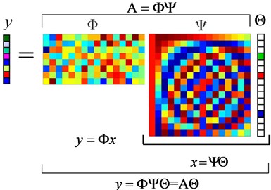
The compressed measurements can be represented in matrix form as Fig. 1. Owing to that the vector $\mathbf{\Theta }$ is sparse, and then the number of the unknowns in Eq. (4) will be reduced greatly so that it is possible to recover $\mathbf{\Theta }$ from $\mathbf{y}$. In order to reconstruct the sparse vector $\mathbf{\Theta }$, Candès and Tao presented and also proved that the $\mathbf{A}$ mentioned above must satisfy Restricted Isometry Property (RIP) [6, 21], and then Baraniuk proposed the idea that the irrelevance between the observation matrix $\mathbf{\Phi }$ with the dictionary matrix $\mathbf{\Psi }$ was the equivalent conditions of RIP [22]. In case that these conditions satisfied, then we can reconstruct sparse representation coefficient vector $\mathbf{\Theta }$ according to the Eq. (4). After the vector $\mathbf{\Theta }$ being obtained, then the original signal $\mathbf{x}$ can be easily recovered based on the Eq. (3). There have many kinds of algorithms to achieve the signal reconstruction, specifically in reference [23-33], etc. in detail. The Matching Pursuit (MP) algorithm will be used to reconstruct signals in our paper [23].

Fig. 1Matrix representation to the compressed measurements

In the previous introduction, the original signal $\mathbf{x}$ is represented sparsely on the dictionary with orthogonal basis. However, this kind of dictionary has limited capacity to the signal sparse representation. Therefore, other types of the dictionaries such as a variety of over-complete dictionaries are often used in practice. According to the difference of the applications, over-complete dictionaries can be divided into two categories: fixed dictionaries which can be used for non-specific signals and trained dictionaries which only used for specific signal. Generally speaking, the fixed dictionary can be used for many different kinds of signals, but it is difficult to decompose the signal very sparsely and the signal representation error would be large. While the trained dictionary can decompose the signal very sparsely since the structure and characteristics information of the training samples is used in dictionary learning process, therefore, the signal sparse representation result can be very good. However, this kind of dictionaries can be used only for the signals which have the same state with the training samples. The most frequently used dictionary learning methods are the MOD (Method of Optimal Directions) [34, 35] and the KSVD (K-Singular Value Decomposition) method [36, 37], and so on. In this paper, the over-complete dictionary on which the signals corresponded to the bearing normal state can be represented sparsely will be trained by the K-SVD method.

3. Fault detection method

For the acquisition of the bearing vibration signal, we denote the collected high-dimensional signal by $\mathbf{x}\in {\mathbf{R}}^N$ based on the traditional Nyquist sampling theorem. While the low-dimensional compressed measurements is denoted by $\mathbf{y}\in {\mathbf{R}}^M$ based on the compressed sampling theory. According to the compressed sensing theory, a high-dimensional signal $\mathbf{x}$ should correspond to a one-to-one low-dimensional signal $\mathbf{y}$ (shown in Fig. 2). If we denote the observation matrix corresponded to the compressed sampling system by $\mathbf{\Phi }\in {\mathbf{R}}^{M\times N}$, then we can get $\mathbf{y}=\mathbf{\Phi }\mathbf{x}$.

We define ${\mathbf{D}}_{normal}$ as the over-complete dictionary trained by dictionary learning method with the bearing historical vibration data corresponded to normal state. This dictionary can be used in sparse representation for the signals in normal state, but not available for the signals in fault state. Expanding the high-dimensional signal $\mathbf{x}$ on the dictionary ${\mathbf{D}}_{normal}$ as:

where $\mathbf{c}$ is the expansion coefficient vector. According to the relation between $\mathbf{x}$ and $\mathbf{y}$, as $\mathbf{y}=\mathbf{\Phi }\mathbf{x}$, we can get:

Fig. 2The relationship between the traditional sampling and compressed sampling

When the vibration signal $\mathbf{x}$ is in normal state, it can be decomposed sparsely on the dictionary ${\mathbf{D}}_{normal}$. In this case, the coefficient vector $\mathbf{c}$ would be sparse, and it is possible to solve $\mathbf{c}$ from the compressed signal $\mathbf{y}$. Defining ${\mathit{}\tilde{\mathbf{c}}}_{normal}$ as the estimate of the coefficient vector $\mathbf{c}$, then the representation error of the compressed signal $\mathbf{y}$ can be calculated as:

In this case, the error ${\mathbf{\delta }}_{normal}$ should be relatively small. Ideally, it should be close to zero.

When the vibration signal x is in fault state, considering that the dictionary ${\mathbf{D}}_{normal}$ is trained using the data in normal state, therefore, it is hard to decompose the signal $\mathbf{x}$ sparsely. In this case, it should be unable to get a sparse coefficient vector c from the compressed measurements $\mathbf{y}$. As the way we solve ${\mathit{}\tilde{\mathbf{c}}}_{normal}$ in the case with normal state, the estimate of the coefficient vector $\mathbf{c}$ can be obtained as ${\tilde{\mathbf{c}}}_{fault}$. Then the representation error of the compressed signal $\mathbf{y}$ can be calculated as:

Therefore, compared to ${\mathbf{\delta }}_{fault}$, the value of ${\mathbf{\delta }}_{fault}$ should be more great.

According to the analysis above, the bearing fault detection can be achieved just using a small amount of compressed measurements directly, which based on the fact that the representation error of the compressed signal $\mathbf{y}$ in normal state is smaller than that in fault state. The process of the fault detection is shown in Fig. 3, and the corresponding steps are as follows:

1) Acquiring the high-dimensional vibration signals when the bearing works in normal state. The set of these signals can be denoted by $\left\{\mathbf{t}|\mathbf{t}\in {\mathbf{R}}^N\right\}$, which will be used as the training samples;

2) Training the over-complete dictionary ${\mathbf{D}}_{normal}$ with the training samples $\left\{\mathbf{t}|\mathbf{t}\in {\mathbf{R}}^N\right\}$;

3) Acquiring the low-dimensional vibration signals $\mathbf{y}\in {\mathbf{R}}^M$ by compressed sampling. Taking $\mathbf{\Phi }\in {\mathbf{R}}^{M\times N}$as the observation matrix, then the high-dimensional signal corresponded to low-dimensional signal $\mathbf{y}$ can be denoted by $\mathbf{x}\in {\mathbf{R}}^N$, and $\mathbf{y}=\mathbf{\Phi }\mathbf{x}$;

4) Setting the threshold (${\mathbf{\delta }}_0$) of the representation error;

5) Calculating the representation error $\mathbf{\delta }$ of the low-dimensional compressed signal $\mathbf{y}$ on dictionary ${\mathbf{D}}_{normal}$, viz. ${\mathbf{\delta }=‖\mathbf{y}-{\mathbf{\Phi }\bullet \mathbf{D}}_{normal}\bullet \tilde{\mathbf{c}}‖}_2$, where $\tilde{\mathbf{c}}$ estimates the expansion coefficient vector of the compressed signal $\mathbf{y}$ on dictionary ${\mathbf{D}}_{normal}$;

6) Estimating the state of the bearing:

In the case that the representation error $\mathbf{\delta }$ is more than the threshold ${\mathbf{\delta }}_0$, then the bearing is determined in fault state.

In the case that the representation error $\mathbf{\delta }$ is less than or equal to the threshold ${\mathbf{\delta }}_0$, then the bearing is determined in normal state.

As can be seen from the fault detection process, the effectiveness of the proposed method is mainly related to the following factors: the principle to determine the fault, the signal reconstruction algorithm and the compressed sampling way and so on. The signal reconstruction algorithm is used to solve the expansion coefficient vector $\tilde{\mathbf{c}}$, and the MP algorithm will be used in this paper. Accordingly, the main parameters which affect the fault detection results include the threshold (${\mathbf{\delta }}_0$) of the signal representation error, the sparsity set in MP algorithm, the amount ($M$) of the compressed measurements and the type of the observation matrix $\mathbf{\Phi }$. In next section, the impacts of these parameters to the fault detection results will be analyzed respectively.

Fig. 3The flow chart of the proposed bearing fault detection method

4. Experimental tests

The proposed fault detection method is validated using the vibration signals from the 6205-2RS JEK SKF deep groove ball bearings (data sources from [38], and the signal sampling frequency is 12 K). The data used in our tests can be divided into two types: the training samples used in dictionary learning and the test samples used for the fault detection validation. The signals sampled in traditional way should be high-dimensional. For dictionary learning, the high-dimensional samples can be used directly. While the test samples should be low-dimensional, in our tests, they will be obtained by simulating the compressed sampling. Defining $\mathbf{\Phi }\in {\mathbf{R}}^{M\times N}$ as the observation matrix, then each high-dimensional signal has $N$ data points and each low-dimensional signal has $M$ data points. In our tests, we set $N$ as 512.

The vibration signals of the bearing in normal state are taken as the training samples, which can be used to training the dictionary ${\mathbf{D}}_{normal}$. There are 20480 signals contained in the training samples, and the data length of each signal is 512. These samples can be divided into four groups and each group contains 5120 signals according to different motor speeds and loads, which are shown in Table 1 below.

Then the over-complete dictionaries ${\mathbf{D}}_{normal}$ corresponded to the normal state can be trained by the K-SVD dictionary learning method using the training samples in Table 1. The parameters in dictionary learning are set as follows. The quantity of atoms is set to 1024. The sparsity is set to 10. The number of loops is set to 20, and the initial dictionary is selected from the training samples.

The original high-dimensional test samples contain 800 signals corresponded to normal state and 1200 signals corresponded to fault states. The fault can be divided into three categories: the inner ring fault, the outer ring fault and the rolling element fault. For each type of fault, we acquire 400 signals. In accordance with different motor speeds and loads, the test samples corresponded to each bearing state contain four groups of signals, as shown in Table 2 below. The faults were designed as single point in inner ring, outer ring and rolling element, which were introduced to the test bearings using electro-discharge machining with fault diameter of 0.021 inches and fault depth of 0.011 inches.

Taking the Gaussian random matrix [39] as the observation matrix in compressed sensing, and setting the amount ($M$) of the compressed measurements as 40, then we can obtained the low-dimensional observations corresponded to the original test samples shown in Table 2. In our proposed method, the bearing states can be determined just using these low-dimensional observations directly. The expansion coefficients vector is solved by the MP algorithm. Setting the sparsity of the coefficients vector as 10, then the fault detection results with different error thresholds are calculated and shown in Fig. 4. The test results can be described using fault detection rate and false alarm rate. The fault detection rate characterizes the ratio of the number of the samples identified as fault state accurately to the number of all the fault samples used in test. The false alarm rate describes the ratio of the number of the samples recognized as fault state which actually should be normal state to the number of all the normal state samples used in test.

It can be seen from Fig. 4 that the bearing fault detection can be achieved effectively when setting a proper error threshold, and we can get a higher fault detection rate with a very low false alarm rate. Compared to the traditional high-dimensional signal with 512 data points, we can get a satisfying detection result just using the compressed signal with 40 data points, which demonstrates the effectiveness of the proposed method.

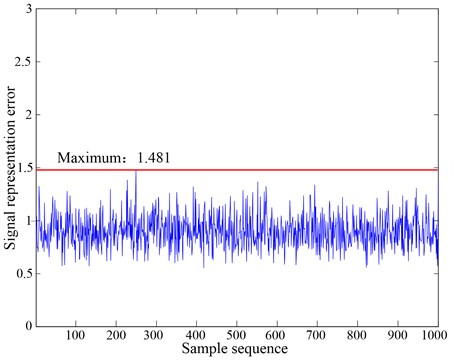
The test results in Fig. 4 also show us a fact that the detection results would be affected by the error threshold directly, therefore, setting a reasonable threshold appears to be particularly important. The error threshold can be set by referring to the prior knowledge. We can select some training samples randomly in Table 1, taking 1000 signals for instance, and then the corresponding low-dimensional signal can be obtained by simulating the compressed sampling. The sampling way for these training samples is the same with that for the test samples. The parameters set here are also the same with that in fault detection. The representation errors of these low-dimensional training samples on the dictionary ${\mathbf{D}}_{normal}$ are solved and the results are shown in Fig. 5. We suggest that the error threshold can be set as the values slightly larger than the maximum of the data in Fig. 5. For example, if we set the error threshold as 1.6, then the fault detection result will be good referring to the Fig. 4, which indicating that we have set an appropriate threshold. In other cases, we can also select an appropriate threshold by referring to the way described above.

Fig. 4The bearing fault detection results with different error thresholds (M= 40)

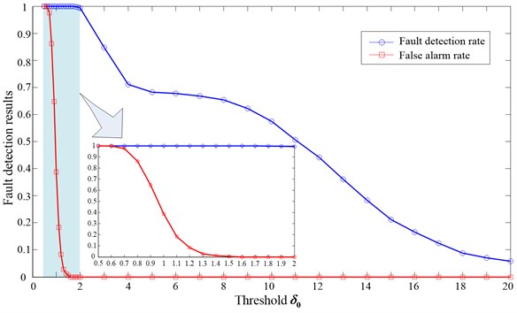
Fig. 5The representation errors of some low-dimensional samples on Dnormal

In the previous analysis, we just used 40 compressed measurements in fault detection. The following analysis will focus on the bearing fault detection results with different amount of compressed measurements. For the cases with different amount of measurements, the threshold will always be set by the principle as ${\mathbf{\delta }}_0=1.2{\mathbf{\delta }}_{max}$, where ${\mathbf{\delta }}_{max}$ is defined as the maximal representation error in the results like Fig. 5. In this test, the Gaussian random matrix is taken as the observation matrix. The expansion coefficients vector is solved by MP algorithm and the sparsity of the coefficients vector is set as 10. Then the fault detection rates and false alarm rates with different amount ($M$) of the compressed measurements are calculated and the results are shown in Fig. 6.

As can be seen from Fig. 6, setting the error threshold based on the above-described principle, the false alarm rate can be very low no matter how many the amount of compressed measurements is. With the increase of the measurements, the fault detection rate will improve gradually, and then finally tend to one, which should be consistent with the theoretical results. With the increase of the compressed observations, more information of the bearing state will be contained in the low-dimensional signal, which benefits the fault detection consequentially.

Fig. 6The fault detection results in different amount of the compressed measurements

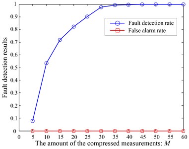
Fig. 7The fault detection results when setting different sparsity in MP algorithm

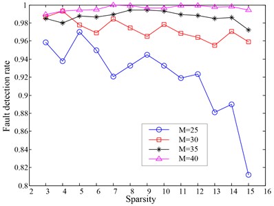
In the above tests, the sparsity of the expansion coefficients vector in MP algorithm was always set as 10, meaning that the number of the atoms involved in signal decomposition would be 10. In fact, this value is not limited to 10. The fault detection results corresponded to different sparsity in MP algorithm will be calculated and analyzed. In our tests, the thresholds are always set by the principle as ${\mathbf{\delta }}_0=1.2{\mathbf{\delta }}_{max}$, where ${\mathbf{\delta }}_{max}$ is defined as the maximal representation error in the results like Fig. 5. Taking the Gaussian random matrix as the observation matrix, and the number ($M$) of the compressed measurements is set as 25, 30, 35 and 40 respectively, then the corresponding fault detection rates when setting different sparsity in MP algorithm are solved. The fault detection results are shown in Fig. 7. Considering that the false alarm rates can be always guaranteed in a very low level when setting the proper thresholds, therefore, we just plot the fault detection rates in Fig. 7.

As can be seen from Fig. 7, for fewer compressed measurements, the fault detection rates will fluctuate obviously with the spasity increasing. Moreover, the general trend would be downward. While for more measurements, the detection rates would be higher and stabilized. In summary, if we obtained fewer compressed measurements, then a small sparsity in MP algorithm should be appropriate. If we get more measurements, then the spasity can be set relatively larger. However, we must notice that the sparsity should not be very large, for a too large sparsity will bring in the increasing of the computation, which should be a disadvantage to bearing fault detection. Generally speaking, the sparsity in MP algorithm can be set as the value which is equal to the sparsity in training the dictionary ${\mathbf{D}}_{normal}$, just as what we did in this paper.

In the experimental tests of this section, we obtained the compressed measurements by taking the Gaussian random matrix as the observation matrix. Actually, different compressed sampling system will correspond to different observation matrix, and we can also use other compressed sampling ways. To validate our proposed method with different compressed sampling ways, we will analyze and compare the fault detection results in several typical compressed sampling ways (based on Gaussian random matrix, partial orthogonal matrix [6] and Toeplitz and circulant matrix [40] respectively). As that in above tests, the thresholds are always set by the principle as ${\mathbf{\delta }}_0=\text{1.2}{\mathbf{\delta }}_{max}$, where ${\mathbf{\delta }}_{max}$ is defined as the maximal representation error in the results like Fig. 5. The expansion coefficients vector is solved by MP algorithm and the sparsity is set as 10. Then the fault detection rates when using different observation matrix are calculated and the results are shown in Fig. 8. Considering that the false alarm rates can be always guaranteed in a very low level when setting the proper thresholds, therefore, we just plot the fault detection rates in Fig. 8.

It can be seen from Fig. 8 that with the increasing of the compressed measurements, the fault detection results will improve gradually in all of the three compressed sampling ways. Moreover, when $M$ is larger than 35, the detection rate will gradually approach one. This results show that the proposed method is effective when taking any one of the three compressed sampling ways. The Fig. 8 also indicates that the fault detection result when using Toeplitz and circulant matrix is better than that using other two observation matrix. While the other two compressed sampling ways have the similar ability in bearing fault detecting with our propose method.

Fig. 8The fault detection results corresponded to different observation matrix

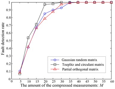
Fig. 9The fault detection results corresponded to different noise level

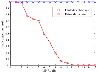
In practice, the compressed signals are often contaminated by external noise, which will affect the fault detection results. Therefore, we will discuss how the proposed method can withstand external noise. As that in above tests, the thresholds are always set by the principle as ${\mathbf{\delta }}_0=\text{1.2}{\mathbf{\delta }}_{max}$, where ${\mathbf{\delta }}_{max}$ is defined as the maximal representation error in the results like Fig. 5. The expansion coefficients vector is solved by MP algorithm and the sparsity is set as 10. Suppose the compressed signals were contaminated by white Gaussian noise, and then the fault detection results corresponded to different SNR (signal-to-noise ratio) are calculated and the results are shown in Fig. 9.

It can be seen from Fig. 9 that the noise has little effect on the fault detection rate, which will be stable at a very high level no matter how strong the noise is. While the false alarm rate is affected by the noise obviously. With the decreasing of the SNR of the compressed signals, the false alarm rate will increase gradually. When the SNR is equal to 0 dB, the false alarm rate will be 100 %, which means that all the signals in normal state actually will be determined in fault state. When the SNR of the signals is more than 11 dB, the fault detection rate will tend to 100 %, and the false alarm rate will drop to 0. Therefore, weak noise will not obviously affect the fault detection results of the proposed method, while strong noise will have great effect on the false alarm rate.

5. Conclusions

A bearing fault detection method based on the low-dimensional compressed measurements is proposed in this paper. In the proposed method, it is not necessary to reconstruct the original high-dimensional signals. The bearing fault detection can be achieved using a small amount of compressed measurements directly, which based on the difference of the representation errors between the compressed signals in normal state and in fault state on a over-complete dictionary. The main parameters which affect the fault detection results include the threshold of signal representation error, the sparsity set in MP algorithm, the amount of the compressed measurements and the type of the observation matrix. The impacts of these parameters to the fault detection results are analyzed respectively, and the effectiveness of the proposed method in bearing fault detecting is validated. The error threshold can be set by referring to the prior knowledge. The sparsity in MP algorithm can be set as the value which is equal to the sparsity in dictionary learning. More compressed measurements are propitious to the bearing fault detection. The Toeplitz and circulant matrix in compressed sampling has better performance in fault detection. Weak noise will not obviously affect the fault detection results of the proposed method, while strong noise will have great effect on the false alarm rate.

In the proposed method, the bearing fault detection can be achieved just using the over-complete dictionary corresponded to bearing normal state. Actually, if we can collect the vibration signals in different fault states, then the over-complete dictionaries corresponded to different fault types can be trained, which will be the foundations for the fault recognition. Therefore, how to use the low-dimensional compressed measurements directly to achieve the bearing fault diagnosis will be the interests of our further research.