Autoregressive modeling approach of vibration data for bearing fault diagnosis in electric motors

1. Introduction

Induction motors are one of the frequently used electrical drives in industrial processes and predictive maintenance of these motors is an important issue to ensure safe, reliable and economic operation of the industrial processes. The information related to fault features have to be known previously to take necessary and timely maintenance actions. The statistical studies on the distribution of failure causes of induction motors have shown that 41 % of failures are caused from bearing related faults. This is the highest percentage among other type of faults such as stator related and rotor related faults [1-5].

For predictive maintenance studies it is necessary to know fault features. To extract bearing fault features, signal based methods such as statistical and spectral analysis techniques are used frequently [2-5]. In these methods fault features are investigated on the acquired data and compared with their baseline values.

Autoregressive (AR) modeling is a parametric method which represents the signal as a linear combination of its previous values plus an error term. This method has relatively simple numerical algorithms and has been widely applied e.g. to nuclear power plants, rolling mill processes, biomedical systems [6-8]. It is used for performing system identification, feature extraction, anomaly detection, diagnosis, classification and forecasting. AR modeling is also employed in rotating machines to detect gear and bearing faults [9-15].

The motor vibration signals contain wide range of sharp peaks rather than deep valleys in their power spectral density variations [9, 12, 16]. The AR method is appropriate to detect those peaks whereas the other well known linear parametric methods such as moving average (MA) and autoregressive integrated moving average (ARIMA) methods are appropriate for spectra which has deep valleys or mixed of them.

The main motivation of this study is to perform fault detection based upon the variations of model parameters. In this manner neural and fuzzy methods which can also be used in time series modeling are not appropriate methods due their black-box structures.

In this study, AR models of the vibration signals are established using the data acquired from healthy and gradually aged induction motor. Variation of model coefficients, modeling errors and spectra of original and its AR model are compared to investigate effectiveness of AR modeling technique for detecting bearing fault.

2. AR modeling method

A wide sense AR process of order $p$ may be generated by filtering white noise $v\left(n\right)$ which has variance ${\sigma }_v^2$ with an all-pole filter shown in Fig. 1 [16, 17].

Fig. 1AR modeling

The filter can be defined by a difference equation and transfer function as below:

The filter coefficients that produce the best approximation $\widehat{x}\left(n\right)$ to $x\left(n\right)$ are determined using the autocorrelation sequence of the AR process satisfying the Yule-Walker equations, which are:

where $\delta \left(k\right)$ is the unit sample sequence. Thus given the autocorrelations $r_x\left(k\right)$ for $k=$0, 1,…, $p$ these equations can be solved for the AR coefficients $a_k$ and ${\sigma }_v$. In most applications $r_x\left(k\right)$ is unknown and estimated from a sample realization of the process. Given $x\left(n\right)$ for $0\le n\le N$, where $N$ is the number of samples, $r_x\left(k\right)$ is estimated using the sample autocorrelation:

Power Spectral Density (PSD) of the signal can be estimated using AR model parameters as below:

AR model order can be determined according to Akaike’s Information Criteria (AIC) as follows:

After finding the AR model coefficients, the signal is predicted using these coefficients thereby forming a moving average process as shown in Fig. 2. The signal is predicted by:

The residual or prediction error is given as:

Fig. 2Prediction

Another approach for extracting the information about the frequency features of a random signal is to transform the signal to the frequency domain by computing the discrete Fourier transform. For a block of data of length $N$ samples, the transform at frequency $m∆f$ is given by:

where $∆f$ is the frequency resolution and $∆t$ is the data-sampling interval. The auto-power spectral density of $x\left(t\right)$ is estimated as:

3. Experimental data

Bearing fault is formed artificially by the shaft current technique which includes running the motor for 30 minutes with the motor rotating at no load and externally applied shaft current of 27 A at 30 V alternating current. This form of damage is called as fluting damage, and bearing components get damaged caused by electrical sparking [3-5, 11]. After the fluting aging, the motor is aged also thermally and chemically.

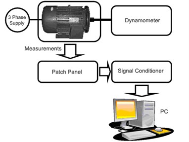
The vibration signals analyzed in this study are obtained by the experimental setup and data acquisition system shown in Fig. 3 in order to get fault characteristics. Here the test motor is put on a motor performance test platform and the measurements are taken after each aging cycle. Seven aging cycles is performed before the motor is broken. During this test procedure, the motor vibration data with a sampling frequency of 12 kHz is acquired at 100 % load condition for one healthy and seven gradually aged cases of the motor. Vibration measurement is taken by the accelerometer which is closer to the bearing at process-end side of the motor.

Fig. 3Motor load testing and data acquisition system

4. AR modeling of vibration signals and feature extraction

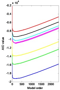
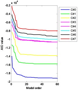
In order to search fault characteristics related to bearing fault, AR modeling technique is applied to the vibration signal which is acquired from the healthy and gradually aged cases of motor. Vibration data is collected for 10 s duration and total data length is 120000 samples. Fig. 4 shows the variation of AIC values for each aging cycle as a function of model order. Here the number of samples is taken as 2400 samples which correspond to measurement time of 0.2 s. The model orders which makes AIC value minimum for each cycle is given in the Table 1.

Fig. 4Variation of AIC values with AR model order in the range of 1 to 2400 a) and b) its zoomed version

a)

b)

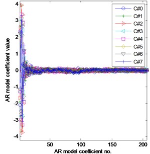
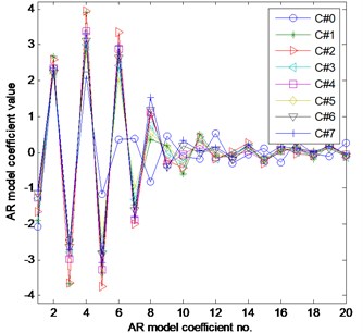
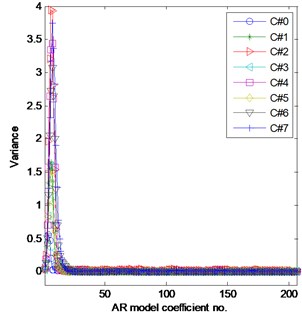
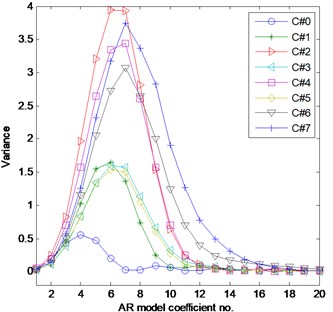
Fig. 5 presents the variation of AR coefficients with respect to model orders for one healthy and seven aged cases of the motor. Here the model order is taken as 207 since it is the maximum number given in Table 1. In this figure the 10 s duration data is segmented into 0.2 s duration which makes 50 segments each containing 2400 samples. For each segment AR coefficients are computed and averaged. Fig. 6 shows the variance of AR coefficients over 50 segments for each model order.

Fig. 5Variation of AR coefficients with AR model order in the range of 1 to 200 a) and b) its zoomed version

a)

b)

Although AIC proposes a high model order number, it can be observed from the Fig. 5 and Fig. 6 that as model order gets bigger the coefficients and their variances are getting smaller. Therefore the model order is accepted as 60 to show progress of bearing fault adequately. Moreover similar results are obtained with the model order found from AIC.

Fig. 6Variance of AR coefficients with AR model order in the range of 1 to 200 a) and b) its zoomed version

a)

b)

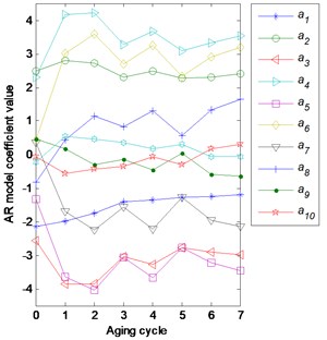
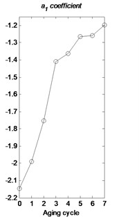
Fig. 7 shows the first 10 AR coefficients namely $a_1$, $a_2$,…, $a_{10}$ which are dominant compared to other remaining 50 AR coefficients for each aging cycle. It is seen that only the $a_1$ coefficient is continuously increasing as the aging progresses.

Fig. 7Variation of first 10 AR coefficients a) and the a1 coefficient b) with aging cycles

a)

b)

Fig. 8Variance of white noise input to drive the AR models

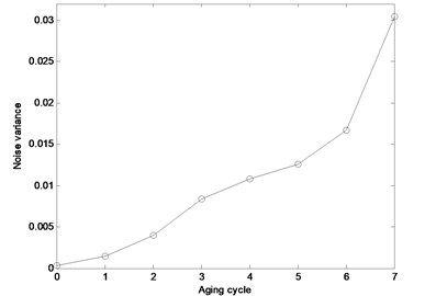
White noise is used as input to get AR model of vibration signal time series. The variance ${\sigma }_v^2$ of the white noise increases with aging as shown in Fig. 8.

After the determination of model order and AR model coefficients, the signals are predicted. Fig. 9 shows original signal and its AR model for the healthy and faulty vibration signals. Fig. 10 shows the error or residual for all aging cycles to see progress of aging. This time domain plots show the prediction errors are increased with aging.

Fig. 9Original vibration signals and their predictions by AR method for healthy and faulty cases

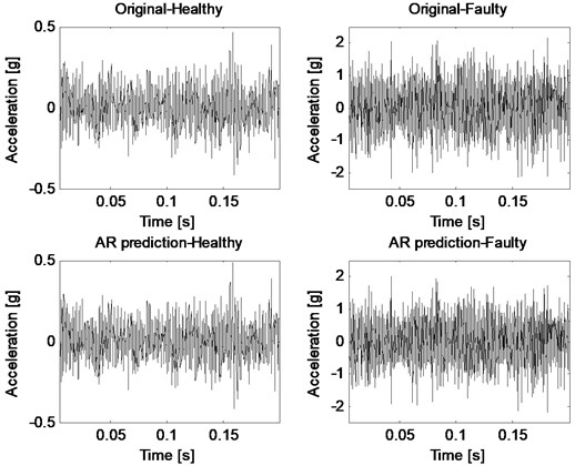
Fig. 10Prediction errors for each aging cycles

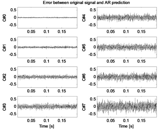
Fig. 11 shows the variance of original and predicted signals by AR method for each aging cycles. It is seen that the trend is similar to each other and it can be said that although there is small difference for some cycles AR prediction performance is acceptable to reflect aging.

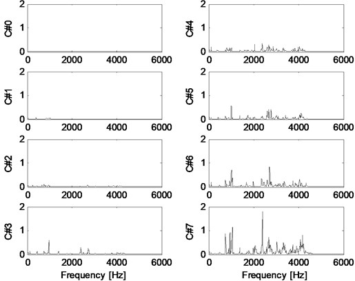
Fig. 12 shows the PSD variations of original vibration signals and their AR predictions for healthy and faulty cases. Fig. 13 shows the absolute error between PSD of original signal and PSD of their AR prediction for all aging cycles. This frequency domain plots show that the energy of this error at higher frequencies gets bigger with aging. From the literature it is known that bearing fluting damage shows itself in a frequency range of 1.5-4 kHz in the spectrum of vibration signal which is compatible with the results in this study.

Fig. 11Variance of original and predicted signals

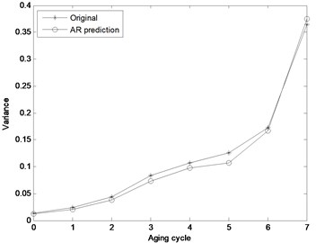
Fig. 12PSD of original vibration signals and their predictions by AR method for healthy and faulty cases

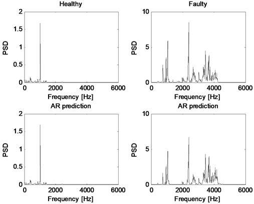
Fig. 13Absolute value of the error between the PSDs of the original signal and its AR prediction for each aging cycle

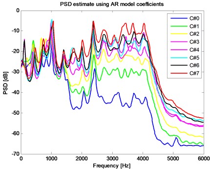
Also the PSD of predicted signals can be estimated by AR model coefficients as shown in Fig. 14. It is seen that the energy of predicted signals by AR method is increased in the frequency range 1.5-4 kHz with aging. It verifies that the AR method can model the data sufficiently with only sixty AR coefficients.

Fig. 14PSD estimate using AR model coefficients

5. Conclusions

In this study effectiveness of autoregressive (AR) modeling method is investigated for extracting bearing fault characteristics. The main reasons for choosing the AR method for time series modeling are the possibility to analyze the model parameters, and promising for vibration signal which have spectrum with sharp peaks. Therefore AR models of motor vibration signals are determined for healthy and gradually aged cases of the induction motor which is subjected to bearing damage artificially. The sixtieth order model is chosen to construct AR models of vibration signals. The first AR coefficient and variance of white noise input to drive the AR model is increased with the aging. Both time domain and frequency domain analysis of original vibration signals and their predictions by AR method give noticeable difference to detect bearing fault. It is seen that the residuals computed in time domain gets bigger as the aging progresses. Also in the frequency domain, the energy of the error computed as the absolute difference between PSDs of original vibration signals and their AR predictions is increased with the aging at the higher frequency region of the spectrum.