An approach for tool health assessment using the Mahalanobis-Taguchi system based on WPT-AR

1. Introduction

In a modern machining system, tool health assessment systems are necessary to ensure high quality production and prevent downtime of mechanical tools as a result of catastrophic failures [1]. Tool health status directly affects the surface finish and dimensional accuracy of a product. Thus, tool health assessment is essential in machining operations [2].

One challenge in effective tool health assessment is selecting a proper feature space that can reflect comprehensive performance [3]. Nowadays, the tool vibration signals usually display strong nonlinear, non-Gaussian and non-stationary features because of the influence of the non-linear factors including clearance, friction, stiffness and so on, so it is difficult to extract a proper feature space which can accurately recognize the working condition of the tools.

The Autoregressive (AR) model is a practical method with simple calculations. It can extract the fault feature of the vibration signals effectively without a requirement of constructing a mathematical model and studying the fault mechanism of the system [4, 5]. Baillie and Mathew used the coefficients of AR model as the input features of an artificial neural network to realize correct classification of the bearing faults [6]. Ocak and Loparo also used the coefficients of AR model as features and adopted hidden Markov model (HMM) to classify different kinds of bearing abnormalities [7]. Weixiang Zhao and Cristina E. Davis demonstrated the distinct advantages of an AR model based feature extraction method for the classification of the chromatography data with time shifts [8]. These applications prove that the autoregressive model is effective to characterize the features of the vibration signal, and it is demonstrated that the coefficients of AR model are very sensitive to condition changes. However, as a model to characterize the stationary time series, estimation of the AR parameters may not be available for nonlinear and non-stationary signals [9]. Aim at this problem, in this paper, the feature vectors of the tool vibration signal are extracted with the combination of wavelet packet transform (WPT) and AR model. Compared with common time-frequency analysis methods, such as Wigner-Ville distributions (WVD), the short time Fourier transformation (STFT), the wavelet transform (WT), etc., the WPT has particular advantages for characterizing signals with a complete multi-level decomposition in both time and frequency domains. Meanwhile, the WPT has particular advantages in extracting features that combine nonlinear and non-stationary characteristics, which is crucial for nonlinear and non-stationary vibration signal [4]. Thus, the WPT and AR models are integrated to ensure better efficacy in the fault feature extraction. Since the singular values are the intrinsic features of a feature vector matrix and have good stability [10], the SVD technique is further developed in this study to decompose the feature vector matrices and obtain singular values.

After extracting feature vectors, a large amount of data can be collected for processes analysis, but another challenge of realizing effective tool health assessment is how to deal effectively with the vast amount of data and build an intelligent assessment model.

The Mahalanobis-Taguchi system (MTS), introduced by G. Taguchi, is a prediction and diagnosis method which is used to analyze data patterns in multivariate systems [11]. It is a pattern information technology, which has been used in different applications to make quantitative decisions by constructing a multivariate measurement scale. In the MTS approach, Mahalanobis distance (MD) is used to measure the degree of abnormality of patterns, whereas the Taguchi methods which utilize orthogonal arrays (OA), and signal-to-noise ratio (S/N), are used to evaluate the accuracy of predictions, and to optimize the system [12].The benefits of MTS as a pattern recognition tool can be summarized as follows [13, 14]: (1) It is a robust methodology that is insensitive to variations in multidimensional systems; (2) It can handle many different types of data sets and effectively consolidates the data into a useful metric; (3) Implementation of MTS requires limited knowledge of statistics; (4) It relies typically on simple arithmetic, contextual knowledge, and intuition; (5) It employs the Taguchi methods to determine the key features and reduce the rest; (6) Its success has been demonstrated in various practical applications. In this study, MTS is employed to provide a computational scheme based on the MD, and the key features are extracted using Taguchi methods.

2. Methodology

2.4. Health assessment method based on WPT-AR and MTS

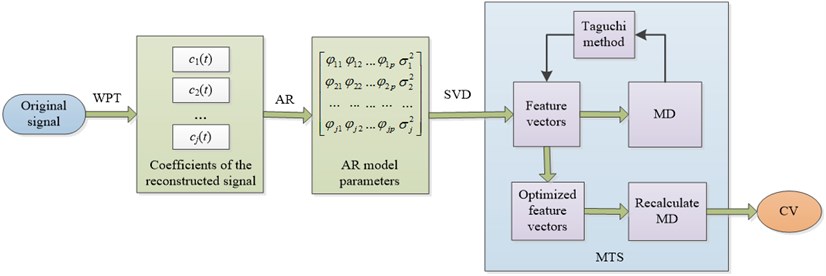
As mentioned, the proposed health assessment scheme can be summarized as shown in Fig. 1.

Fig. 1Scheme of the proposed health assessment method

The procedure can be divided into two main parts:

1) WPT-AR based feature extraction

The tool vibration signal can be decomposed to $2^n$ sub-bands with different frequencies by $n$-level WPT. Coefficients of the reconstructed signal can be defined as $c_1\left(t\right)\text{,}{c}_2\left(t\right)\text{,...,}{c}_j\left(t\right)$ ($j=2^n$), each of which implies different characteristic scale information. Therefore, the characteristics of the tool vibration signal can be obtained by extracting the characteristics of $c_1\left(t\right)\text{,}{c}_2\left(t\right)\text{,...,}{c}_j\left(t\right)$. The AR model for each coefficient $c_i\left(t\right)$ is constructed as:

11

$c_i\left(t\right)={\phi }_{i1}{c}_i\left(t-1\right)+{\phi }_{i2}{c}_i\left(t-2\right)+\dots +{\phi }_{ip}{c}_i\left(t-p\right)+e_i\left(t\right)=\sum _{k=1}^p{\phi }_{ik}{c}_i\left(t-k\right)+e_i\left(t\right),$

where ${\phi }_{ik}$ ($k=$ 1, 2,…, $p$) and $p$, respectively, are the $k$th model parameters and model order of the AR model of the ith coefficient; $e_i\left(t\right)$ is the remnant of the model, a white noise sequence with zero mean value and variance ${\sigma }_i^2$ [10]. As the parameters ${\phi }_{ik}$ ($k=$1, 2,…, $p$) can reflect the inherent characteristics of a tool vibrating system and the variance of the remnant ${\sigma }_i^2$ is tightly related with the output characteristics of the system, ${\phi }_{ik}$ ($k=$1, 2,…, $p$) and ${\sigma }_i^2$ can be chosen as feature vectors $A_i=[{\phi }_{i1},{\phi }_{i2},\dots ,{\phi }_{ip},{\sigma }_i^2]$ to identify the tool condition in the milling machine [5]. Thereafter, the singular value decomposition (SVD) method is used to decompose the feature vector matrices and obtain singular values [20].

2) Health assessment

After the feature extraction, the MDs between the testing data and the benchmark space composed of the normal training data are determined as follows:

12

$M{D}_j=\frac{1}{k}{x}_j^T·R^{-1}·x_j,$

where $R^{-1}$ is the inverse of the correlation matrix $R$, which contains correlation coefficients between the variables, $x_j$ is the column vector of standardized variables, $M{D}_j$ is the $MD$ for the $j$th observation, and $k$ is the number of characteristics.

Then, the Taguchi method is employed to optimize the $n$-dimensional feature vector. The orthogonal table is established, and the larger-the-better signal-to-noise ratio is calculated. By comparing the average signal-to-noise ratio between Level 1 ($t_1$) and Level 2 ($t_2$) of each characteristic, the principal characteristics are extracted and the redundant features are reduced. With the identified key features, the MDs are recalculated for health assessment and finally converted into CVs, thereby achieving the health condition assessment.

3. Case study

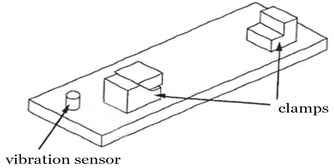
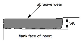
The data in this study are sampled by a vibration sensor that measured runs on a milling machine. Fig. 2(a) shows the mounting position of the vibration sensor. Tool wear occurs in different forms. In our experiments, we measured the flank wear VB as a generally accepted parameter for evaluating tool wear, as shown in Fig. 2(b). Two experiments with cut depth of 1.5 mm feed rate of 0.25 mm/rev, and cut depth of 0.75 mm feed rate of 0.25 mm/rev were chosen as example 1 and 2. Cast iron is used as the material. Here, we mainly focus on example 1.

Fig. 2a) Mounting position of the vibration sensor, b) Measure of flank wear VB

a)

b)

3.1. Feature extraction

In example 1, a total of 40 samples have been acquired under normal conditions. The first 30 normal samples are used to construct the normal space and the others are used for testing. Among the samples, 10 have a VB of 0.18 mm, and these samples are also acquired for the testing process. Fig. 3 illustrates a sample of WPT results of the normal vibration signal.

Fig. 3A sample of WPT results of the normal tool signal

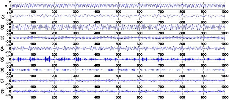
Table 2Extracted singular values for model training

Number	State	1	2	3	4	5	6	7	8
1	Normal condition	12.6596	11.6476	2.0088	1.4113	0.8029	0.2152	0.1703	0.1328
2		12.6885	11.6316	1.9789	1.3542	0.7955	0.2255	0.1741	0.1356
3		12.6753	11.6344	1.9908	1.3871	0.8048	0.2168	0.1707	0.1353
4		12.6696	11.6170	1.9811	1.3794	0.8038	0.2169	0.1782	0.1333
5		12.6602	11.6247	1.9926	1.3935	0.8071	0.2120	0.1749	0.1238
6		12.7062	11.6544	1.9851	1.3911	0.7982	0.2188	0.1701	0.1367
7		12.6904	11.6415	1.9842	1.3958	0.8019	0.2133	0.1681	0.1425
8		12.7053	11.6178	1.9692	1.3776	0.8057	0.2307	0.1792	0.1370

The AR model is constructed for each coefficient of the reconstructed signal $c_1\left(t\right)\text{,}{c}_2\left(t\right)\text{,...}\text{,}{c}_8\left(t\right)$. In this case, the order, m, is determined as 7, so the AR parameters ${\phi }_{ik}$ ($k=$1, 2,… , 7) and ${\sigma }_i^2$ are chosen to form the initial feature matrix. Then, SVD is employed to obtain an 8-dimensional feature vector of singular values. Some of the extracted singular values are listed in Tables 2 and 3.

Table 3Extracted characteristic vectors for testing

Number	State	1	2	3	4	5	6	7	8
1	Normal condition	12.7162	11.6418	1.9826	1.3946	0.8055	0.2281	0.1677	0.1303
2		12.7171	11.6276	1.9775	1.3630	0.8071	0.2273	0.1749	0.1199
3		12.7272	11.6938	1.9952	1.3934	0.8066	0.2262	0.1592	0.1271
4		12.7631	11.6370	1.9657	1.3776	0.8092	0.2355	0.1642	0.1317
1	Worn condition	12.6851	11.7671	1.8333	1.3133	0.7581	0.4003	0.1844	0.1161
2		12.6662	11.7570	1.8504	1.3368	0.7604	0.4170	0.1797	0.1168
3		12.6434	11.7149	1.8185	1.3063	0.7584	0.3785	0.1872	0.1193
4		12.6591	11.7237	1.8676	1.3518	0.7586	0.3786	0.1816	0.1210

3.2. Health assessment based on MTS

3.2.1. MD calculation

After feature extraction, the $MD$ values of the testing samples under normal and worn conditions are calculated. Table 4 presents the experimental results. These results prove that the MD method is highly effective for fault diagnosis.

Table 4Mean, minimum, and maximum of MDs

	Normal condition	Worn condition
Mean	2.6454	337.1591
Min-max	1.0153-5.3637	252.4657-408.8422

3.2.2. Optimization based on the Taguchi method

The extracted feature vector is constructed by 8-dimensional singular values. Therefore, the $L_9\left(2^8\right)$ OA is employed to identify the useless characteristics. We used 30 samples of normal conditions ($VB=$0 mm) and 10 samples of worn conditions ($VB=$0.18 mm) in the Taguchi experiment. The results are reported in Table 5.

Table 5Results of Taguchi method

	1	2	3	4	5	6	7	8	SNR
1	1	1	1	1	1	1	1	1	21.24
2	1	1	1	1	1	2	2	2	20.84
3	1	1	2	2	2	1	1	1	15.75
4	1	2	1	2	2	1	2	2	21.86
5	1	2	2	1	2	2	1	2	15.94
6	1	2	2	2	1	2	2	1	17.92
7	2	1	2	2	1	1	2	2	19.23
8	2	1	2	1	2	2	2	1	13.14
9	2	1	1	2	2	2	1	2	13.98
$t_1$	18.93	17.36	19.48	17.79	19.81	19.52	16.73	17.01
$t_2$	15.45	18.57	16.40	17.75	16.13	16.36	18.60	18.37
$t_1-t_2$	3.48	–1.21	3.08	0.05	3.68	3.15	–1.87	–1.35
Useful	Y	N	Y	Y	Y	Y	N	N

According to the rules of the Taguchi method, the 2nd, 7th, and 8th singular values should be excluded as redundant factors. With the identified key features, the $MD$ values for all of the testing datasets were recalculated. Table 6 presents a comparison between the initial and optimized MDs for each dataset. The result confirms that the Taguchi methods are highly effective in characteristic optimization.

Table 6Comparison between initial and optimized MDs

	Normal condition
	Initial	Optimized
Mean	2.6454	2.0733
Min–max	1.0153-5.3637	0.8284-3.5922
	Worn condition
	Initial	Optimized
Mean	337.1591	130.8750
Min-max	252.4657-408.8422	112.5295-155.6077

3.2.3. Health assessment

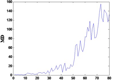
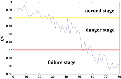
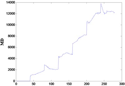
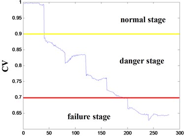
A total of 80 samples from example 1 and 280 samples from example 2 are chosen to verify the effectiveness of the proposed method. In example 1, every 10 samples are in the same $VB$. The $MD$ values and CVs of each group are calculated, as shown in Fig. 4.

Blue curve in Fig. 5 indicates the health degradation of the tool. The first 20 samples with CVs above 0.9 can be considered as “normal stage”, which shows that the tool is in good health condition. Thereafter, the MDs increase while the CVs decrease, and the tool is considered to be at “danger stage”. Once the $CV$ drops below the threshold of 0.7, the tool is considered to be at “failure stage”.

Fig. 4MDs and CVs of the tools in example 1

a)

b)

In example 2, every 40 samples are in the same $VB$. The $MD$ values and CVs of each group are shown in Fig. 5. The blue curve shows the same trend as in example 1. The first 40 samples are in the “normal stage”, with CVs above 0.9. As the tool health degrading, the CVs fall at the same time, which can be considered as “danger stage”. The last 80 samples are in the “failure stage”, with CVs bellow 0.7.

Thus, the health condition of the tool can be coincidentally represented by the $CV$. The experiment results demonstrate that the proposed health assessment method based on WPT-AR and MTS performs efficiently.

Fig. 5MDs and CVs of the tools in example 2

a)

b)

4. Conclusions

This paper presents a health assessment method for tools in milling machine using MTS based on WPT-AR. Targeting nonlinear and non-stationary signals from the milling process, the WPT-AR method is employed in feature extraction and forms the initial feature matrix. Singular values of this feature matrix are obtained via SVD. Then, MTS is employed for health assessment, which has been verified by vibration signals obtained from the milling machining process. Generally speaking, the proposed approach has two benefits. First, it extracts the suitable features that evidently reflect the health state of tools because the combination of WPT and AR prevents drawbacks in processing nonlinear and non-stationary signals. Second, it is a reliable real-time multivariate analytical method that offers a systematic way to determine the principal characteristics through MTS.