Model validation of aeroelastic system for robust flutter prediction

2.1. Framework of model validation

The generic problem of model validation can be described as follows: If the given uncertain model or the model set can reproduce the measured testing input and output data under the influence of unknown but norm bounded exogenous disturbance and noise, the uncertain model is considered to be a model validating uncertainty set, i. e. the model is unfalsified. Model validation, which is based on certain identification mechanism and optimization algorithm, is a process to determine the magnitudes of uncertainties through measured input and output testing data. In fact, there is no model that can be completely validated by finite testing data, because new measurement may violate the current model. Thus, we can only prove that the model is not invalid, i.e. unfalsified [24].

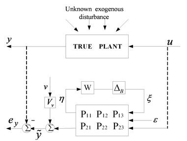
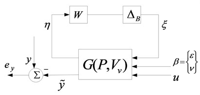
Fig. 1Model validation framework (a) and canonical form (b)

(a)

(b)

The LFT framework of model validation and its canonical form is shown as Fig. 1. The inputs $u$ and the outputs $y$ are the actual signal of the true plant which can be measured in testing, while the simulated output signal of the plant model $\tilde{y}$ is a sum of responses exited by noise, disturbances, and known input signal $u$.${\mathbf{e}}_{\mathbf{y}}=\mathbf{y}-\tilde{\mathbf{y}}$ is the error between measured and simulated output and $\mathbf{\Delta }$ is the structured uncertainty model defined by Equation (1). Diagonal matrix $\mathbf{W}$ denotes the weightings of uncertainties and each diagonal element represents the bound of the corresponding uncertainty. $\mathbf{\eta }$ and $\mathbf{\xi }$ are the internal fictitious signals that relate the uncertainties and the nominal plant. In order to simulate the actual testing environment, measurement noise $v$ of the output and exogenous disturbances $\epsilon$, which affects the system through the controlled input channel or a separate path, are introduced. Signals $\epsilon$ and $v$ are $L_2$ norm bounded, so the independent bounds on the two signals $‖\epsilon ‖\le 1$ and $\Vert v\Vert \le 1$ are assumed. ${\mathbf{P}}_{ij}$, $i=1,2$; $j=1,2,3$ are the transfer function matrices and consist of an augment nominal model $\mathbf{P}$. A noise transfer function matrix $V_v$ and a disturbance transfer function matrix $V_{\epsilon }$ are designed to imbed into the partitioned blocks ${\mathbf{P}}_{12}$ and ${\mathbf{P}}_{22}$ of the augmented nominal plant $\mathbf{P}$. Both transfer functions are assumed driven by unknown but bounded independent random signals. For convenience, both exogenous disturbances $\epsilon$ and $v$ are combined into a single disturbance vector $\text{β}=\left\{\begin{array}{c}\epsilon \\ v\end{array}\right\}$, which is approximately norm bounded by $‖\mathbf{\beta }‖\le 1$ for mathematical simplicity. For each discrete frequency point, the actual disturbance signal can be considered as $\widehat{\text{β}}\approx {\mathbf{V}}_{\beta }\text{β}$, where ${\mathbf{V}}_{\beta }=\left[\begin{array}{c}{\mathbf{V}}_{\epsilon }\\ 0\end{array}\begin{array}{c}0\\ {\mathbf{V}}_v\end{array}\right]$. Then after the combined disturbance signal $\mathbf{\beta }$ is applied, the framework diagram of Fig. 1(a) can be simplified to a more concise form shown as Fig. 1(b), where the transfer function matrices $\mathbf{G}=\left[\begin{array}{c}{\mathbf{G}}_{11}{\mathbf{G}}_{12}{\mathbf{G}}_{13}\\ {\mathbf{G}}_{21}{\mathbf{G}}_{22}{\mathbf{G}}_{23}\end{array}\right]$ are determined by $\mathbf{P}$ and ${\mathbf{V}}_v$. Note also that it is typical in many applications that $u$ is assumed known, so if the output error $e_y=y-\tilde{y}=0$ is satisfied, the input error is also equal to zero. Therefore, only considering output error constraint is sufficient for the presented application.

Define the structured uncertainty:

where $\tau$ is the number of uncertainty block and $F_i$ denotes the real number filed $R$ or the complex numbers field $C$. A corresponding set of bounded structured uncertainty is defined by:

where the elements of the diagonal matrix:

are the scaling radii applied to the blocks of the structured uncertainty of which the unit ball is defined by $\overline{\sigma }\left({\mathbf{\Delta }}_{\mathit{B}}\right)\le 1$.

The transfer relationships obtained from Fig. 1 is shown as follows:

where ${\mathbf{e}}_y^0=\mathbf{y}-{\mathbf{G}}_{23}\mathbf{u}$ is the output error of the nominal plant. It is seen from Eq. (7) that the structured uncertainty term ${\mathbf{G}}_{21}\mathbf{\xi }$ and exogenous disturbances term ${\mathbf{G}}_{22}\mathbf{\beta }$ could share the output error ${\mathbf{e}}_y^0$ jointly. If the output data of the actual system is distorted by the disturbance $\mathbf{\beta }$ and the influences are not considered in the model validation framework, the identified uncertainty magnitudes would be overly large which will result in a conservative robust flutter prediction.

Before performing model validation, the transfer function matrix ${\mathbf{V}}_{\beta }$ needs to be determined. Assume that, the mean square value and variance of the true measurement noise $v_{true}$ have been obtained as the prior informations. Then white gauss noise with the same mean square value and variance is simulated to generate signal $v_{sim}$, which can be used to determine transfer function matrix ${\mathbf{V}}_v$ [18]:

where $N$ denotes an $N-$point DFT sample used in model validation with sampling interval $T_s$. $n_{out}$ is the number of noise channels and $s\left[v_{sim}^2\right]$ is the power spectra of the simulated signal $v_{sim}$.

2.2. Parameterization of model validating sets

Only if ${\mathbf{e}}_y=0$, the norm bounded combined disturbance $\mathbf{\beta }$ ($‖\mathbf{\beta }‖\le 1$) and uncertainty output signal $\mathbf{\xi }$ can reproduce the given input and output measurements, which means the given model set is not invalidated. Define $\mathbf{M}=[{\mathbf{G}}_{21},{\mathbf{G}}_{22}]$, then the following equations can be obtained:

In the above equations, ${\mathbf{N}}_M$ is a matrix of which the columns consist of a basis for $\text{Ker}\left(\mathbf{M}\right)$ and the symbol ${(.)}_{\beta }$ denotes the sub-matrix which is associated with $\mathbf{\beta }$, i.e. the corresponding row vectors extracted from matrices ${\mathbf{M}}^{+}$ and ${\mathbf{N}}_M$ according to the dimension of $\mathbf{\beta }$ in Eq. (10). Parameter $\mathbf{\theta }$ is an arbitrary vector with appropriate dimension.

The condition for the existence of a model validating set can be stated as follows: there exists $\mathbf{\theta }$ such that Eq. (9) and the inequality $‖\mathbf{\beta }‖=‖{\left({\mathbf{M}}^{+}\right)}_{\beta }{\mathbf{e}}_y^0+{\left({\mathbf{N}}_M\right)}_{\beta }\mathbf{\theta }‖\le 1$ are satisfied. In order to find the parameter $\mathbf{\theta }$ that satisfies $‖\mathbf{\beta }‖\le 1$, ${\left({\mathbf{N}}_M\right)}_{\beta }$ is decomposed through singular value decomposition (SVD). Then $\mathbf{\theta }$ can be parameterized by the new introduced parameter vectors $\mathbf{\phi }$ and $\mathbf{\psi }$ and is shown as:

In this decomposition, ${\mathbf{T}}_1$, ${\mathbf{T}}_2$, ${\mathbf{U}}_1$, ${\mathbf{U}}_2$ are unitary, ${\mathbf{\Sigma }}_1$ is diagonal and nonsingular, and the block matrix partitioning are conformal. Symbol $H$ denotes conjugate transpose. $\mathbf{\phi }$ and $\mathbf{\psi }$ are arbitrary and satisfy $‖\mathbf{\phi }‖\le b_0=\sqrt{1-‖{\mathbf{T}}_2^H{\left({\mathbf{M}}^{+}\right)}_{\beta }{\mathbf{e}}_y^0‖}$ and $n_{\phi }+n_{\psi }=\text{dim}\left[\text{Ker}\right(\mathbf{M}\left)\right]$, where $n_{\phi }$ and $n_{\psi }$ are dimensions of the vectors. Correlate Eq. (13), (10) with (5), the pair of signals $(\xi ,\eta )$ are given by the parameterization:

where ${\mathbf{\eta }}_0$ and ${\mathbf{\xi }}_0$ are constant vectors and ${\mathbf{I}}_{n_{\xi }}$ is an identity matrix with a dimension equals to that of $\mathbf{\xi }$. $\mathbf{\Omega }$ is defined as $\mathbf{\Omega }={\mathbf{N}}_M\left[{\mathbf{U}}_1{\mathbf{U}}_2\right]\left[\begin{array}{cc}{\mathbf{\Sigma }}_1^{-1}& 0\\ 0& {\mathbf{I}}_{\Omega }\end{array}\right]$, where ${\mathit{I}}_{\Omega }$ is an identity matrix, of which the dimension is determined by $n_{\phi }+n_{\psi }-\text{rank}{\left({\mathbf{N}}_M\right)}_{\beta }$.

According to Eq. (4), the signals $\xi$ and $\eta$ have to be consistent with their transfer relationship through the uncertainty structure $\mathbf{\Delta }$. Colum vectors $({\mathbf{\xi }}_1,...,{\mathbf{\xi }}_{\mathrm{\tau }})$ and $({\mathbf{\eta }}_1,...,{\mathbf{\eta }}_{\mathrm{\tau }})$ are the partitioning of vectors $\mathbf{\xi }$ and $\mathbf{\eta }$ that conforms to the block diagonal partition of $\mathbf{\Delta }$ in Eq. (1) and their norm ratios determine the uncertainty magnitudes $w_i$. For repeated and/or real scalar blocks, the collinearity condition is:

and for full complex blocks, another condition Eq. (17) has to be satisfied:

The parameterization of the pair of signals $(\xi ,\eta )$ is not unique which means that the validating model with the capability to reproduce the available data is not unique. In order to reduce the conservatism of the results, it is necessary to reasonably design the proportion distribution of the uncertainty weightings/radii $w_i$ and to find the model validating set with the smallest uncertainty magnitudes. A positive factor $x$ is introduced in order to simultaneously scale the uncertainty magnitudes according to the designed proportion. Thus, $x{w}_i$ becomes the real uncertainty magnitude. Specifically, a constrained nonlinear optimization process with $\psi$ and $\phi$ as the design variables is used to find a minimal positive $x$ such that $P_{xW}$ is a model validating set. So Eq. (17) can be written as:

Thus, the problems can be formulated as a constrained nonlinear optimization problem which is described as follow: the the design variables are $x$, $\mathbf{\psi }$, $\mathbf{\phi }$ and ${\delta }_i$; the constraint conditions are Eq. (16), Eq. (18), $x>0,$$‖\mathbf{\phi }‖\le b_0$ and $\left|{\delta }_i\right|\le x\left|w_i\right|$; the objective is to find the smallest $x$. First, determine the proportion distribution of uncertainty weightings which is obtained by analyzing the priori knowledge and should reflects the true uncertainty mechanism. Second, select initial values of the design variables according to the constraints. Then the problem can be solved with a sequential quadratic programming which is provided by the Optimization Toolbox of MATLAB [25]. After finding the smallest $x$, $x{w}_i$ will characterize the uncertainty magnitude and $P_{xW}$ will be the desired model validation result.

3.1. Equation of motion

The governing equation of a generic aeroelastic system is:

where $\mathbf{M}$, $\mathbf{C}$ and $\mathbf{K}$ are the modal mass, structural modal damping and modal stiffness matrices, respectively; $\mathbf{X}$ is the vector of generalized coordinates, $q$ is the dynamic pressure and $\mathbf{Q}\left(ik,Ma\right)$ is the generalized aerodynamic influence coefficient (AIC) matrix, which depends on Mach number $Ma$ and reduced frequency $k$.

The AIC can be obtained by several aerodynamic theories, such as doublet lattice method, ZONA 51 and piston theory et al. In this paper, the doublet lattice method (DLM) was adopted for subsonic unsteady aerodynamic force computation. In aeroelastic community, DLM is a universally acknowledged method for subsonic unsteady aerodynamic force calculation. It was first proposed in 1969 [26], and developed as a classical aerodynamic model for flutter analysis. Several aeroelastic analysis softwares, such as MSC. Flight loads and Dynamics [27], ZONA ZAERO [28], employ DLM or the improved version as one of the core aerodynamic modules.

Based on small disturbance hypothesis, DLM solves the linearized potential flow equation and obtains the aerodynamic forces under the condition that the aerodynamic panel oscillates harmonically. The aerodynamic panel is divided into small trapezoidal lifting elements, where the horse-shoe vortex are assigned to each grid to represent steady flow, and acceleration potential doublets are placed in the 1/4 chord length to simulate additional terms of unsteady aerodynamics. To satisfy the Kutta condition at trailing edge, the middle point at 3/4 chord length of each grid is chosen as the control point, for which the boundary conditions must be satisfied.

The AIC is a set of matrices which are computed for distinct values of reduced frequency. Thus, in order to compute AIC for any desired frequency point conveniently and rapidly and perform time domain analysis, the aerodynamic forces obtained in frequency-domain have to be transformed into time-domain representations. Several methods often referred to as rational function approximations, have been developed to describe the unsteady aerodynamic forces analytically. This paper uses Roger’s formulation [29] to represent the aerodynamic forces which is shown in Equation (20):

In Eq. (20), ${\mathbf{Q}}_1$, ${\mathbf{Q}}_2$, ${\mathbf{Q}}_3$ and ${\mathbf{E}}_i$ are coefficient matrices which are solved by approximation algorithm; $\overline{s}$ is defined as $\overline{s}=ik=i\frac{\omega b}{V}$, where $\omega$ is the frequency of vibration, $b$ is the reference semichord and $V$ is airspeed; $r_i$ are the poles used to describe the effects of aerodynamic lags. The formulation used in this paper considers four lag terms to represent the unsteady aerodynamic effects.

3.2. Uncertainty modeling

For complex systems such as a real aircraft, the sources and structures of uncertainty are highly diversified and difficult to be described. The uncertainties of mass (fuel consumption), damping and unsteady aerodynamic force are the significant sources for aircraft systems and the influences of nonlinearities and unmodeled dynamics are also non-negligible. The additive and multiplicative uncertainties also have distinct characteristics. In this paper, the complex influences of uncertainties being derived from numerous sources and being of several structures are not discussed, because the mechanism of uncertainty commonly depends on the specific problems, of which the identification involves profound understanding of aeroservoelasticity and abundant engineering experiences which are not the main purpose of this paper. The source and structure of the uncertainties are only assumed to demonstrate the validity of the model validation method and evaluate the robust flutter predictions. In the presented study, the parametric uncertainties of damping and stiffness are modeled for structure, and both parametric uncertainty and the unmodeled dynamics of unsteady aerodynamic forces are considered and discussed respectively. The uncertainties are formulated as follows:

where ${\mathbf{C}}_0$ and ${\mathbf{K}}_0$ are the nominal matrices, ${\mathbf{C}}_1$ and ${\mathbf{K}}_1$ are used to choose the type of uncertainty [30]. For example, ${\mathbf{C}}_1={\mathbf{C}}_0$ means the multiplying uncertainty and ${\mathbf{C}}_1=\mathbf{I}$ indicates the additive uncertainty. Since $\mathbf{C}$, $\mathbf{K}$ are modal damping and modal stiffness, they are all diagonal matrices. Consequently, ${\mathbf{\Delta }=\mathbf{\Delta }}_C{\mathbf{W}}_C$ and $\mathbf{\Delta }={\mathbf{\Delta }}_K{\mathbf{W}}_K$ are repeated scalar blocks or real scalar blocks.

Unsteady aerodynamic uncertainties might be the most significant source and have a strong influence on the dynamic behavior of the aeroelastic system [16]. $\mathbf{Q}(ik,Ma)$ can be obtained by appropriate aerodynamic theory such as Doublet-Lattice Method (DLM). But various simplifications and assumptions are used in the theoretical models which lead to difficulties in accurately modeling of wing tip and control surface aerodynamics. An elaborative modeling of aerodynamic uncertainty is developed by Borglund and discussed in detail in [16]. Here, we just use the method and procedures to model aerodynamic uncertainty without detailed presentation. If the aerodynamic uncertainty is considered as unmodeled dynamics, the description can be formulated as:

where ${\mathbf{Q}}_0$ is the nominal aerodynamic influence matrix, ${\mathbf{\Delta }}_Q$ is the unknown full complex block and ${‖{\mathbf{\Delta }}_Q‖}_{\infty }\le 1$. ${\mathbf{W}}_Q=w_Q{\mathbf{I}}_m$ is the weightings used to scale the unity-bound operator and $m$ is the order of nominal plant. If the aerodynamic uncertainty is considered to be parametric, a concise form that accounts for the contributions of modal aerodynamic to the entire generalized aerodynamic uncertainty is adopted and represented as repeated scalar blocks. The parametric uncertainty is written as:

where ${\mathbf{E}}_j$ is a matrix of which the elements are zero except $e_{jj}=1$; $n$ is number of the mode that is considered to have remarkable influences on aerodynamic uncertainty. ${\mathbf{\Delta }}_j={\delta }_j{\mathbf{I}}_m$ and ${\mathbf{W}}_j=w_j{\mathbf{I}}_m$ are also defined.

Substituting the uncertainty expression Eq. (21) and Eq. (22) into the equation of motion Eq. (19), the obtained equation can be written as:

Define ${\mathbf{C}}_1\dot{\mathbf{X}}={\mathbf{\eta }}_C\text{,}$${\mathbf{K}}_1\mathbf{X}={\mathbf{\eta }}_K\text{,}$$q\mathbf{X}={\mathbf{\eta }}_Q\text{,}$${\mathbf{\Delta }}_C{\mathbf{W}}_C{\mathbf{\eta }}_C={\mathbf{\xi }}_C\text{,}$${\mathbf{\Delta }}_K{\mathbf{W}}_K{\mathbf{\eta }}_K={\mathbf{\xi }}_K$ and ${\mathbf{\Delta }}_Q{\mathbf{W}}_Q{\mathit{\eta }}_Q={\mathbf{\xi }}_Q$, a concise equation can be obtained as:

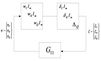
Perform Laplace Transformation for Eq. (25), and compute the transfer function from $\mathbf{\xi }$ to $\mathbf{X}$ and $\mathbf{X}$ to $\mathbf{\eta }$, the transfer function ${\mathbf{G}}_{11}$ between $\mathbf{\xi }$ and $\mathbf{\eta }$ is obtained. Then the $\mu$-analysis loop for robust flutter computation with full complex blocks is shown as Fig. 2.

Fig. 2μ-analysis loop with full complex blocks

Substituting the uncertainty expression Eq. (21) and Eq. (23) into the equation of motion Eq. (19), the uncertain aeroelastic equation can be written as:

Define ${\mathbf{C}}_1\dot{\mathbf{X}}={\mathbf{\eta }}_C\text{,}$${\mathbf{K}}_1\mathbf{X}={\mathbf{\eta }}_K\text{,}$$q{\mathbf{Q}}_0{\mathbf{E}}_j\mathbf{X}={\mathbf{\eta }}_{Q_j}\text{,}$${\mathbf{\Delta }}_C{\mathbf{W}}_C{\mathbf{\eta }}_C={\mathbf{\xi }}_C\text{,}$${\mathbf{\Delta }}_K{\mathbf{W}}_K{\mathbf{\eta }}_K={\mathbf{\xi }}_K$ and ${\mathbf{\Delta }}_j{\mathbf{W}}_j{\mathbf{\eta }}_{Q_j}={\mathbf{\xi }}_{Q_j}$, one can obtain:

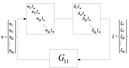
The transfer function matrix ${\mathbf{G}}_{11}$ between $\mathbf{\xi }$ and $\mathbf{\eta }$ is also obtained and the $\mu$-analysis loop for robust flutter computation with repeated scalar blocks is shown as Fig. 3.

Fig. 3μ-analysis loop with repeated scalar blocks

4.1. Straight wing model

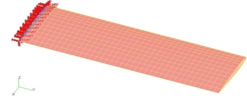
The finite element model of straight wing with NACA0012 airfoil is modeled using MSC/PATRAN software and is shown in Fig. 4. The unsteady aerodynamic forces are compute for $Mach=\text{0.3}$ by doublet lattice method and the first ten order of modal mass ${\mathbf{M}}_{10}$, modal stiffness ${\mathbf{K}}_{10}$, modal damping ${\mathbf{C}}_{10}$, generalized AIC ${\mathbf{Q}}_{10}$ and mode shape vectors are exported by DMAP techniques [31]. The generalized AIC matrices of different reduced frequency are approximated by Roger method and then the aeroelastic equation can be transformed to time domain. The modal parameters of actual system are designed as ${\mathbf{M}}_{real}={\mathbf{M}}_{10}$, ${\mathbf{C}}_{real}=1.10{\mathbf{C}}_{10}$, ${\mathbf{K}}_{real}=0.95{\mathbf{K}}_{10}$ and the first 5 orders modal parameters ${\mathbf{M}}_0$, ${\mathbf{C}}_0$, ${\mathbf{K}}_0$ and the corresponding generalized AIC matrix ${\mathbf{Q}}_0$ are defined as the nominal model. For structure, the parametric uncertainties of stiffness and damping are considered and for aerodynamics, the uncertainty is considered as parametric uncertainty of modal aerodynamics and unmolded dynamics respectively.

Fig. 4The finite element model of straight wing

The excitation signal is applied to the straight wing model and the response is obtained by mode superposition. The simulated input and output signals are all recorded and used as measured data in flight testing. According to the method and procedures described in previous section, the uncertainties of structure and aerodynamics are modeled and the disturbance and noise which is inevitable in real testing environment are introduced to the model validation framework. Finally, the LFT framework of model validation is established. As mentioned before, model validation requires prior information of the system and uncertainty. This information could be helpful for assigning the weightings of each uncertainty and determining the proportion relationship reasonably. For parametric uncertainty of modal aerodynamics, the studied case considers the first two modes are of more importance and provide primary contributions for aerodynamic uncertainties. This is because the generic flutter is caused by two modes unstable couplings and it is easier to determine the weighting proportion for less parameter. However, how to determine the proportion among several uncertainty weightings is a problem involves the study of interaction mechanism of various uncertainties, deriving from different sources and being of different structures. The main purpose of this paper is to present a model validation method and demonstrate its feasibility and validity, so that study is not included.

If the weighting proportion relationship between each uncertainty $w_C:w_K:w_{Q_1}:w_{Q_2}$ is determined, the scaling factor $x$ is optimized in order to validate the uncertainty model set. In real test, the influence of disturbance and noise is inevitable. If the errors between theoretical model and actual system are entirely ascribed to uncertainties of structure and aerodynamic forces, the magnitudes of uncertainties will be overestimated which would cause a much conservative result of robust flutter prediction. Thus, the influence of disturbance and noise is considered to reduce the conservatism effectively.

The stability of the so-called “actual system” is analyzed by state-space method and flutter speed is obtained as $V_{real}=\text{166}\text{m/s}$, while the flutter speed of the presupposed nominal model is $V_{nom}=\text{170}\text{m/s}$. For case of parametric aerodynamic uncertainty, the weighting proportion relationship is designed as $w_C:w_K:w_{Q_1}:w_{Q_2}=2:1:1:1$. The analysis is considered as three different circumstances and discussed respectively, (a) there is no disturbance and noise in real system testing, i. e. $\mathbf{\epsilon }=\mathbf{v}=0$, which means it is not necessary to introduce signal $\mathbf{\beta }$ to the validation framework and ${\mathbf{V}}_{\beta }=0$ is applied. (b) the influence of disturbance and noise did exist in actual system testing, but the influence is not included for model validation, i. e. ${\mathbf{V}}_{\beta }=0$. (c) the influence of disturbance and noise did exist in real system testing, and this influence is accounted for by simulated signal in the model validation framework, which would share the modeling errors with the uncertainties together. Table 1 displays the model validation results of the parametric uncertainty for sea level. $V_{rob}$ denotes the robust flutter speed and the unit is m/s.

According to the model validation results, the robust flutter speed for the three different circumstances can be calculated by $\mu$ toolbox embedded in MATLAB software [32]. The up bounds of $\mu$ values of different speeds are computed and the flight speed corresponding to $\mu =$1 is defined as the robust flutter speed which is also shown in Table 1.

It can be seen from Table 1 that the robust flutter speeds are lower than the nominal flutter speeds, which demonstrates that the robust flutter boundary takes the uncertainty into consideration and is the flutter speed of the worst-case. The robust flutter speed varies as the uncertainty magnitudes, so different uncertainty magnitudes for the three circumstances, which are obtained by model validation, results in different robust flutter speed.

The weighting proportion of the uncertainties is used for all the three cases, and the results of uncertainty magnitudes and robust flutter speeds are exhibited in Table 1. It is seen that Case (a) is an ideal condition that excludes any disturbance and noise from the actual system and the influence of them is also not considered in model validation. The errors between nominal model and actual system are entirely ascribed to uncertainties and the magnitudes are estimated according to this assumption. But the influence of disturbance and noise is inevitable and even strong in actual system and real test environment. If their influences are not taken into account in model validation, the errors between nominal model and actual system will be entirely undertaken by uncertainty which will result in larger estimation of uncertainty magnitude and conservative robust flutter prediction. Results of Case (b) demonstrate this clearly. The uncertainty magnitudes are much larger than those of Case (a) and the predicted robust flutter speed is also much more conservative. As for Case (c), the terms of disturbance and noise are formulated in model validation framework to represent their influence on actual system in real test environment. Thus, the modeling errors can be commonly shared by uncertainty and disturbance and noise. Model validation should exclude the influence of disturbance and noise as much as possible and identify the uncertainty magnitudes correctly. The consistency of the results of Case (a) and (b) demonstrates the validity of the presented method. It is seen that the presented model validation method can accurately estimate the components of the model errors that are contributed by uncertainty and the rest errors can be considered caused by disturbance and noise.

For Case (c), the influences of different uncertainty weighting proportions on the uncertainty magnitudes obtained by model validation and the subsequently predicted robust flutter speeds are studied and discussed. The proportional relations are set for both two types of aerodynamic uncertainty structures and the robust flutter speeds are also predicted respectively. The results are displayed in the following table, where $V_{rob}$ denotes the robust flutter speed and the unit is m/s.

Comparing the results of the two structure types of aerodynamic uncertainty shown in Table 2, it is seen that aerodynamic uncertainty of parametric form produces little more conservative results, while the unmodeled dynamics descriptions which are expressed by full complex blocks reduce the conservatism of the predicted results. Although the parametric aerodynamic uncertainty represented by repeated scalar blocks could reflect the contribution of modal aerodynamics to the uncertainties and gives a specific physical meaning, the uncertainty structure is fixed, which will lead to a strong constraint for the optimization process. On the other hand, the form of full complex blocks relaxes the constraints on the structure of uncertainty, which will reduce the conservatism of the predicted results.

The weighting proportion also affects the predicted robust flutter speed. Proportional relationship (1) could reflect the prior information accurately, since the proportion is set according to the deviations of the stiffness and damping of the nominal model from the “known actual system”. Therefore, the corresponding results are relatively close to the real flutter speed. Proportional relationship (2) increases the magnitude of damping uncertainty and decreases the magnitudes of stiffness and aerodynamic uncertainties. These variations have a small effect on the predicted robust flutter speed. The results demonstrate that the structural damping has no remarkable influence on flutter speed which is considered as a regular phenomenon and a basic conclusion in aeroelasticity. Proportional relationship (3) and (4) increase the magnitudes of stiffness and aerodynamic uncertainties respectively, and the results indicate that the primary factors that significantly affect the flutter speed are stiffness and aerodynamic uncertainties, especially the aerodynamic uncertainty.

Apparently, if the weighting proportion between the uncertainties is set unreasonable, the predicted results will be excessively conservative. Although it is guaranteed that the actual system can be included in the aeroelastic model set, the prediction will be meaningless. Thus, it is concluded that the prior information about uncertainty, the actual system and the test condition and environment is very important, which can provide the mechanism of uncertainty, influence of various uncertainty on flutter speed and the initial guesses of uncertainty magnitude. Since aerodynamic forces and stiffness have a remarkable influence on flutter speed, it is desired that the magnitudes of aerodynamic and stiffness uncertainties be as small as possible. So the corresponding weighting proportion should be assigned relatively lower. On the other hand, in order to obtain a less conservative prediction, the model errors should be assigned to damping uncertainty as much as possible, which is less sensitive to flutter speed. It is seen from Table 2 that the assignment and trade-off of weighting proportion is of great influences on the final model validation results and robust flutter predictions. How to determine the weighting proportion and subsequently reduce the conservatism of the prediction is a crucial problem of model validation and is worthy of further study.

4.2. Fuselage-wing-store model

In aircraft structure design, the configuration that suspends the external stores, such as missiles and auxiliary fuel tank under the wing is very common. It is well known that the addition and/or modification of external equipment and stores on the aircraft deeply impact its aeroelastic characteristics, which are not fully predictable using linear flutter engineering tools and require flight test to produce a safety operational flight envelope with confidence. The influence of the store on aircraft structure is obvious, which causes dramatic parameter changes of the entire fuselage-wing-store structure. As for aerodynamics, although the wing provides major lifting forces for an aircraft and the stores commonly have slender configuration which does not provide lifting forces directly, the aerodynamic interferences among every aircraft component indeed affect the aerodynamic forces and the flow field. Therefore, the significant influence of fuselage-wing-store aerodynamic interferences on the flutter speed can’t be neglected. This effect proposes challenges for unsteady aerodynamics calculation and flutter analysis. The modeling of external store aerodynamics precisely and concisely is difficult, so it is desirable and reasonable to consider these aerodynamic interferences as aerodynamic uncertainties for robust flutter analysis.

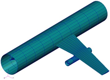
As the geometry is assumed symmetrical, the finite element model of a half of the aircraft with external store for calculating normal modes using MSC/NASTRAN is shown in Fig. 5. The flutter characteristics of the fuselage-wing-store structure with/without aerodynamic interference effects are compared and the influences of aerodynamic interference on aerodynamic forces and flutter speed are discussed. It is assumed that, the aerodynamic influence matrix without interferences is the nominal matrix and the aerodynamic influence matrix of the entire model considering store and fuselage aerodynamic interferences is the true plant matrix. The variations of aerodynamic matrix due to the influences of slender bodies are considered to be unmodeled dynamics with full complex blocks structure. The numerical example established a finite element model of a half simplified aircraft with one external store. The actual system, nominal system and uncertainty description are designed and the input and output signals are simulated as testing data to perform model validation. Robust stability of the uncertain aeroelastic system is analyzed via theory of structured singular value and the robust flutter speed is obtained.

The aerodynamic interference model is shown as Fig. 6. The flow field of the fuselage-wing-store model is treated as laminar flow, implying that flow is attached to the solid wall at all times and no separation is observed. Since the flow velocity is in subsonic regime, shock wave would not appear or is so weak that can be neglected. The unsteady aerodynamic forces of the wing without aerodynamic interferences are computed by doubletlattice method, while the fuselage-wing-store aerodynamic interferences have influences on the flutter speed. To account for this effect, the global fuselage-wing-store aerodynamic forces are computed via subsonic wing-slender interference theory [31], which idealizes bodies (i. e. fuselage and store) as “slender” and “interference” elements in combination. The primary purpose of the slender body elements is to account for the forces arising from the motion of the body, whereas the interference elements are used to account for the interference among all bodies and panels in the same group. This is implemented by providing a surface through which the corresponding boundary conditions are imposed. The aerodynamic interference effects are reflected in the obtained AIC matrices.

Fig. 5The finite element model of fuselage-wing-store model

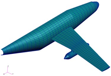
Fig. 6The fuselage-wing-store aerodynamic interferences model

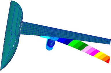
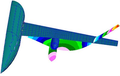
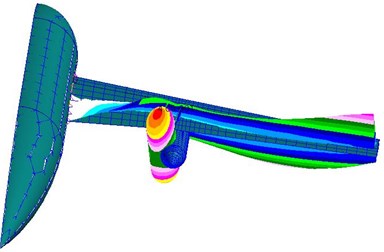
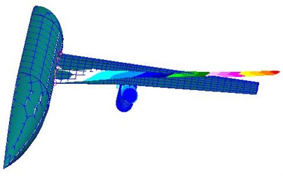
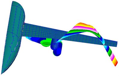
The first five order structural modal parameters and mode shapes and aerodynamic influence coefficient matrices are calculated and exported. Table 3 shows the natural frequencies and Fig. 7 displays the mode shapes. The modal mass $M_5$, stiffness $K_5$, damping $C_5$, generalized AIC matrix $Q_5$ and mode shape vectors are all obtained. Note that, $Q_5$ denotes the generalized AIC matrices with the aerodynamic interferences effects of fuselage and store. The parameters of actual system are set as $M_{real}=M_5$, $C_{real}=C_5$, $K_{real}=K_5$, $Q_{real}=Q_5$ and the nominal model are designed as $M_0=M_5$, $C_0=C_5$, $K_0=K_5$, $Q_0=Q_{wing}$, where $Q_{wing}$ is chosen as the generalized AIC matrix without considering the interferences of store and fuselage. This design means that the structures of actual system and nominal model are the same, whereas the only differences are aerodynamics with/without interferences of fuselage and store. That is to say only uncertainties of unsteady aerodynamic forces are considered. The flutter speeds of actual system and nominal model for sea level are computed by state-space method and the results are $V_{real}=\text{175.0}\text{m/s}$ and $V_{nom}=\text{171.0}\text{m/s}$ respectively.

Excitation signals with exogenous disturbance are applied to the structure and the aeroelastic responses are simulated in noise environment. Both the input and obtained output data are considered as the testing measured data and used for model validation. The aerodynamic uncertainty is modeled according to section 2.2 and the model validation framework of uncertain aeroelastic system is formulated. Since previous numerical example has demonstrated that the model validation method presented in this paper could effectively eliminate the influence of disturbance and noise on the identification of the uncertainty magnitudes, the exogenous disturbance and noise are introduced to simulate the real testing environment and share the modeling errors with uncertainty. The identified aerodynamic uncertainty magnitude is optimized as $W_Q=\text{0.056}$ and the robust flutter speed of the fuselage-wing-store model with an aerodynamic uncertainty is $V_{rob}=\text{166.5}\text{m/s}$ which is predicted according to the model validation result. The $\mu$ values for three different flow velocities are shown in Fig. 8.

Fig. 7The mode shapes of the fuselage-wing-store model

(a)

(b)

(c)

(d)

(e)

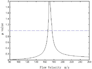
Fig. 9 displays the maximum $\mu$ values of fuselage-wing-store model for a set of values of flow velocities. When the value of flow velocity is lower than the nominal flutter speed, the airspeed associated with $\mu =$1 is the flutter speed of the worst-case, i. e. robust flutter speed. This speed can also be considered as the lower bound of the flutter speed $V_{lower}$, while the airspeed corresponding to another intersection point of $\mu =$1 is defined as the upper bound of the flutter speed $V_{upper}$. The characteristics of $V$-$\mu$ curve are discussed in detail in [33-34]. The flutter speeds of the model set are bounded between $V_{lower}$ and $V_{upper}$, so if the model validation is performed effectively, the real or experimental flutter speed lies within that bound. The lower and upper bounds of flutter speed are $V_{lower}=\text{166.5 m/s}$ and $V_{upper}=\text{176.3 m/s}$. The result indicates that the flutter speed of “actual system” is included in the interval of the bounds, which demonstrates the model validation is effective and the robust flutter prediction is meaningful. Note that the upper bound is very close to the real flutter speed. This closeness indicates that the validation process produces a result with less conservatism. Furthermore, it is found that both lower bound and upper bound provide useful or even important information. To locate the real flutter speed precisely, the interval of bound should be as narrow as possible, which depends on a less conservative result provided by model validation.

Fig. 8The μ value curves of fuselage-wing-store model with aerodynamic uncertainty

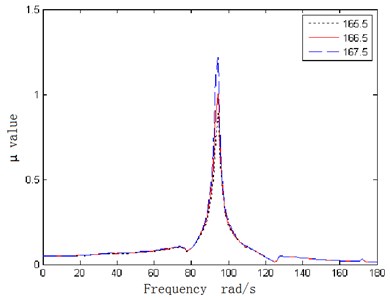
Fig. 9The V-μ curve of fuselage-wing-store model with aerodynamic uncertainty

For aircraft with stores, the aerodynamic interferences of store, the stiffness of pylon between aircraft and store, the span location of store and the variation of mass and gravity center all have certain influences on the flutter characteristics of aircraft. The presented example only considers the influences of the aerodynamic interferences induced by slender bodies of fuselage and store. The interferences of slender bodies on panel aerodynamics are set as unmodeled dynamics and the corresponding uncertainty magnitude is estimated by the model validation procedures presented in this paper. It is observed from the model validation result and the robust flutter prediction that the fuselage-wing-store aerodynamic interferences can be identified as an uncertainty and this manner of treatment is reasonable. Therefore, the influences of fuselage-wing-store aerodynamic interferences on flutter characteristics should be considered as an important factor in flutter analysis.