Abstract
In this article a genetic algorithm optimized Lagrangian support vector machine algorithm and its application in rolling bearing fault diagnosis is introduced. As an effective global optimization method, genetic algorithm is applied to find the optimum multiplier of Lagrangian support vector machine. Synthetic numerical experiments revealed the effectiveness of this genetic algorithm optimized Lagrangian support vector machine as a classifier. Then this classifier is applied to recognize faulty bearings from normal ones. Its performance is compared with that of backpropagation neural network and standard Lagrangian support vector machine. Experimental results show that the classification ability of our classifier is higher and the computing time required to find the separating plane is relative shorter.
1. Introduction
Nowadays there is an explosion in the number of research papers on support vector machines (SVMs) [1-2], which have been successfully applied to a number of areas ranging from expression recognition [3], text categorization [4] to machine fault diagnosis [5-6] and image retrieval [7-8]. These references illustrate the effectiveness of SVM as a classification tool. In SVM, a typical quadratic program problem has to be solved to find the best separating plane. It is a computational very demanding process. O. L. Mangasarian and David R. Musicant (2001) give a fast simple algorithm named Lagrangian support vector machine (LSVM) [9], which is “based on an implicit Lagrangian formulation of the dual of a simple reformulation of the standard quadratic program of a linear support vector machine”. Some other SVM algorithms [10-11] are proposed based on the principle of LSVM. In this article genetic algorithm is applied to find the optimum multiplier of Lagrangian support vector machine for its powerful global optimization ability. Synthetic data tests the effectiveness of the proposed algorithm. Finally, the genetic algorithm based LSVM is applied to diagnose rolling bearing fault and its performance is compared with that of backpropagation network and standard LSVM.
2. Principle of LSVM
Suppose we have given observation points Denote these observations as a matrix . A given diagonal matrix (some of the entries on the main diagonal are +1 and the rest are –1) reveals the membership of each point in the class or . Support vector machine is applied to construct a hyperplane that separates the data into two given classes with maximal margin.
For standard support vector machine, the separating plane with a soft margin can be found by solving the following quadratic program problem:
where is the normal vector of the separating plane, determines the location of the plane relative to the origin, is a non-negative slack variable, controls the tradeoff between errors on training data and margin maximization, , is an unity vector.
The dual to the above quadratic programming problem is the following:
where is the Lagrangian multiplier.
For a support vector machine with nonlinear decision function in non-separable cases, the dual quadratic programming problem is defined as:
where is a kernel function. There are many popular kernels available, some common are polynomial, radial basis function (RBF), neural network kernels and so on.
To find the separating plane, a quadratic programming problem has to be solved, whereas such a problem is complex and computationally very demanding even though there are many existing methods to solve this problem [12] and SVM codes available online such as SVMlight [13] and libSVM [14]. So, O. L. Mangasarian and David R. Musicant (2001) presented a fast simple algorithm named Lagrangian support vector machine (LSVM) [9], in which “two simple changes are made to the standard SVM: (1) the margin between the parallel bounding planes is maximized with respect to both and ; (2) the error is minimized using the 2-norm squared instead of 1-norm”. Based on these changes, a simpler positive definite dual problem with non-negativity constraints replaces the complex quadratic problem of standard SVM.
These two changes lead to the modification of Eq. (2):
where is an identity matrix.
To simplify notation, we define two matrices as followings:
Then Eq. (4) can be rewritten as following:
The optimum can be found by the following iterative expression:
for which we will establish global linear convergence from any start point under the condition:
where denotes the th during recursion, denotes a vector with all of negative components in set to zero.
Like standard SVM, LSVM can also be extended to solve nonlinear classification problems. In nonlinear cases, we give and different definitions:
Just as the linear cases, we can obtain the same iterative scheme as Eq. (7).
3. Genetic algorithm for the optimization of LSVM
The above descriptions reveal that the essence of LSVM is to find an optimum Lagrangian multiplier that minimizes Eq. (6) under constraint condition of . In this section, we try to apply genetic algorithm to solve this problem.
In this article two kinds of genetic algorithm are designed: one is the standard genetic algorithm, named as SGA, and the other is a modified genetic algorithm, denoted by MGA. Both algorithms adopt float encoding and arithmetical crossover operation [15-16]. The difference of these algorithms mainly lies in the mutation operation, which is the main search operation when float encoding is adopted.
Three major steps in executing genetic algorithm (both SGA and MGA) to find the optimum is as following:
A. Generate initial population.
As the dimension of optimization variable equals to the amount of data points to be classified, it is obviously a high dimensional optimization problem. Float encoding is more suitable for this situation. The uniform distribution is used to generate initial individuals of SGA, while individuals of MGA are formed by superimposing perturbation values upon variable which is generated based on the following expression:
B. Iteratively perform the following substeps on the population until the termination criterion is satisfied. The maximum number of generation to be run is determined beforehand.
(1) Assign a fitness value to each individual in the population using the fitness measure.
For a constrained optimization problem defined as Eq. (6), the fitness function with penalty function is constructed to measure the feasibility of individuals:
where is the fitness value of individual is the penalty factor, and is the size of .
(2) Create a new population by applying the following three genetic operations.
Create two new individuals using crossover operation. Suppose , are the selected parents, the sons , are formed based on the following expression:
where is a random number, .
Create a new individual by mutation operation. In SGA, non-uniform mutation operation is adopted. It is operated as following:
Suppose is the selected parent, the component whose definition interval is , is selected to mutate. Then after mutation, the component would change as following:
where variable is a random value in the range , and function rounds to the nearest integer, is the current number of generation, function is defined as following:
where is a random number in the range , is the biggest generation number, is a constant.
In MGA, some knowledge of the function being optimized is put into the operation design. The global search ability of genetic algorithm and local search ability of LSVM are combined to form more powerful search operators. After mutation, the offspring of individual of MGA is the following:
Select better existing individuals to form a new population. In order to avoid premature, ranking selection is adopted by both algorithms.
C. When evolution finished, the best individual of the final population is then the optimum .
4. Synthetic numerical implementation
In this section the effectiveness of proposed algorithms are tested using synthetic data. In order to simplify description, SGA optimized Lagrangian support vector machine is abbreviated as SGA_LSVM, MGA optimized Lagrangian support vector machine is abbreviated as MGA_LSVM.
All of our experiments are run on a personal computer, which utilizes a 3.2 GHz dual-core processor and a maximum of 2GB of memory.
First we try the linear case. For linear case, synthetic data are generated to test our algorithm, shown in Fig. 1. These data points are divided into two data sets: half for building the classifier, the other half for testing the classifier. The parameters for ideal separating plane should be and Table 1 shows the results.
If we set , then obtained by SGA_LSVM is [0.9318, 0.9518], of MGA_LSVM is [1.0364, 1.0163]. and we got are very close to the ideal values. The training correctness and testing correctness reveal the effectiveness of our algorithms as classifier.
Then nonlinear classification ability of our algorithms is tested. Fig. 2 shows the data points for the nonlinear case. Table 2 shows the outputs of our algorithms as classifier with RBF kernel. The results show the feasibility of our algorithms.
Fig. 1Synthetic data for linear case
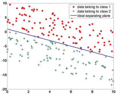
Fig. 2Data points for nonlinear case
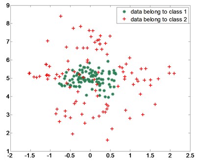
Table 1Results of genetic algorithm based support vector machine
Classifier | Training correctness (%) | Testing correctness (%) | Computing time (sec) | ||
SGA_LSVM | 97 | 98 | 1.823 | [2.4776, 2.5307] | 2.6587 |
MGA_LSVM | 99 | 100 | 0.470 | [0.5465, 0.5358] | 0.5272 |
Table 2Results of our classifier with RBF kernel
Training correctness (%) | Testing correctness (%) | Computing time (sec) | |
SGA_LSVM | 89.1 | 87.2 | 1.549 |
MGA_LSVM | 90.0 | 87.8 | 0.418 |
Table 1 and Table 2 reveal that, for the same problem, MGA_LSVM requires shorter computing time than SGA_LSVM. That means the convergence speed of MGA is higher than that of SGA. The reason lies in the difference of mutation operation. As mentioned above, in MGA, some knowledge of the function being optimized is put into the operation design, thus the convergence speed of MGA is greatly accelerated.
5. Diagnostic practice
In this section, our algorithm is applied to real world problem of rolling bearing faults diagnosis. In order to test the classification ability of our algorithm, backpropagation (BP) network and standard LSVM classifier are also applied to solve the same problem: recognize three types of rolling bearing faults from the normal condition.
In order to verify the performance of proposed method, experiment is conducted on the rolling bearing test rig (Fig. 3). Key phase signal is collected from the input axial with photoelectric sensor. Vibration signals are collected from top and side position of testing bearing. Sampling frequency is set to be 12000 Hz in the experiment. The range of speed fluctuation of the input shaft is 800 rpm-1500 rpm during the experiment.
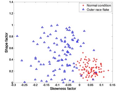
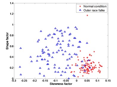
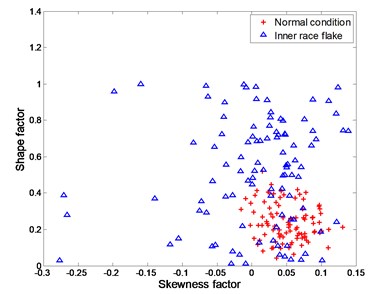
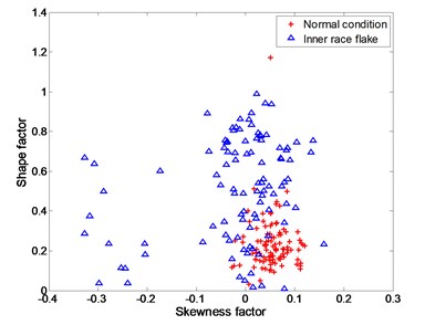
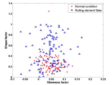
The four working conditions of rolling bearing are: normal condition, inner race flake, outer race flake and rolling element flake. Skewness factor and shape factor are selected as classification features. Fig. 4 – Fig. 6 show the training data and testing data under different working conditions. It is apparently a nonlinear classification problem.
Table 3 – Table 5 show the experimental results obtained by different classifiers. BP is the worst classifier with respect to classification correctness as well as computing time. It performs especially badly when there is a serious aliasing between two classes, such as the case of classifying normal condition and rolling element flake, in which the classification correctness is less than 50 %.
Fig. 3Test rig for rolling bearing experiment
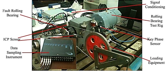
Table 3Comparison of recognition ability and computing time of different classifiers Condition: normal, outer race flake
SGA_LSVM | MGA_LSVM | LSVM | BP | |
Training correctness (%) | 92.5 | 97.5 | 98.5 | 86.5 |
Testing correctness (%) | 91.5 | 94.5 | 92.5 | 85.0 |
Computing time (sec) | 6.213 | 1.236 | 9.591 | 73.955 |
Table 4Comparison of recognition ability and computing time of different classifiers Condition: normal, inner race flake
SGA_LSVM | MGA_LSVM | LSVM | BP | |
Training correctness (%) | 85.5 | 89.0 | 90.0 | 64.0 |
Testing correctness (%) | 84.5 | 86.5 | 86.0 | 62.0 |
Computing time (sec) | 6.108 | 1.326 | 10.188 | 68.450 |
Table 5Comparison of recognition ability and computing time of different classifiers Condition: normal, rolling element flake
SGA_LSVM | MGA_LSVM | LSVM | BP | |
Training correctness (%) | 74.5 | 78.5 | 81.0 | 28.0 |
Testing correctness (%) | 75.5 | 78.5 | 74.0 | 32.5 |
Computing time (sec) | 5.982 | 1.452 | 10.235 | 69.658 |
Fig. 4Experimental data for distinguishing between normal condition and outer race flake
a) training data
b) testing data
Fig. 5Experimental data for distinguishing between normal condition and inner race flake
a) training data
b) testing data
Fig. 6Experimental data for distinguishing between normal condition and rolling element flake
a) training data
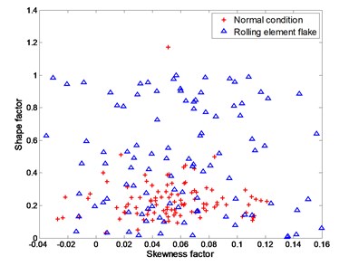
b) testing data
For a classifier, we care more about testing correctness which represent generalization ability of a classifier than training correctness. For the other three classifiers, the classification ability of MGA_LSVM classifier is slightly better than that of standard LSVM, while that of SGA_LSVM is relatively worse. As for computing time, MGA_LSVM requires the shortest computing time, and then the SGA_LSVM, standard LSVM requires the longest time. These observations show that MGA _LSVM performs the best compared with three other classifiers.
6. Conclusion
In this article genetic algorithm is introduced to solve the optimization of Lagrangian support vector machine, and is applied to practice diagnostic problem. Two kinds of genetic algorithm are designed, denoted by SGA and MGA respectively. The operation is described in detail. Synthetic numerical experiments revealed the effectiveness of these two GA optimized LSVM classifiers, it also show that the convergent speed of MGA is faster than that of SGA. Then these classifiers are applied to recognize fault bearings from normal ones. Their performance is compared with that of neural network and standard Lagrangian support vector machine. Experimental results show that MGA_LSVM is the best classifier compared with three other classifiers with respect to both recognition ability and computing time.
References
-
V. Vapnik The Nature of Statistical Learning Theory. Springer Verlag, New York, Inc., USA, 1995.
-
Javier M., Alberto M. Support vector machines with applications. Statistical Science, Vol. 21, Issue 3, 2006, p. 322-336.
-
Yani Z., Jiayou D., Jiatao S. Expression recognition based on genetic algorithm and SVM. Fuzzy Information and Engineering, Vol. 62, 2009, p. 743-751.
-
Taiyue W., Hueimin C. Fuzzy support vector machine for multi-class categorization. Information Processing & Management, Vol. 43, Issue 4, 2007, p. 914-929.
-
Achmad W., Bo S. Y. Support vector machine in machine condition monitoring and fault diagnosis. Mechanical Systems and Signal Processing, Vol. 21, Issue 6, 2007, p. 2560-2574.
-
Junhong Z., Yu L., Feng R. B. Diesel engine valve fault diagnosis based on LMD and SVM. Transactions of CSICE, Vol. 30, Issue 5, 2012, p. 469-473.
-
Jian C., Kong Q. W. Active learning for image retrieval with Co-SVM. Pattern Recognition, Vol. 40, Issue 1, 2007, p. 330-334.
-
Xiaohong S., Jin D., Peijun M. Image retrieval by convex hulls of interest points and SVM-based weighted feedback. Chinese Journal of Computers, Vol. 32, Issue 11, 2009, p. 2221-2228.
-
Mangasarian O. L., David R. Lagrangian support vector machines. Journal of Machine Learning Research, Vol. 9, Issue 1, 2001, p. 161-177.
-
Jae Pil H., Seongkeun P., Euntai K. Dual margin approach on a Lagrangian support vector machine. International Journal of Computer Mathematics, Vol. 88, Issue 4, 2011, p. 695-708.
-
Xiaowei Y., Lei S., Zhifeng H. An extended Lagrangian support vector machine for classifications. Progress in Natural Science, Vol. 14, Issue 6, 2004, p. 519-523.
-
Kristin P., Colin C. Support vector machines: Hype or Hallelujah?. SIGKDD Explorations, Vol. 2, Issue 2, 2000, p. 1-13.
-
Joachims T. SVMlight. http://svmlight.joachims.org/, 2010.
-
Chih C. C., Chih J. L. http://www.csie.ntu.edu.tw/~cjlin/libsvmtools/, 2001.
-
Randy L. H., Sue E. H. Practical Genetic Algorithm. Wiley-Interscience, 2004.
-
Agoston E. E., Smith J. E. Introduction to Evolutionary Computing. Springer, 2008.
About this article
This project was accomplished thanks to the funds of National Natural Science Foundation of China (No. 51175049) and Special Fund for Basic Scientific Research of Central Colleges (No. CHD2011JC025).
