An approach to health assessment for tools in milling machine

2.1. Empirical mode decomposition

EMD is a self-adaptive method to decompose nonlinear and non-stationary signals. The advantage of EMD is that basis functions are derived from the analyzed signal itself. Hence, the signal analysis is adaptive in contrast to the traditional methods where basis functions are fixed. It decomposes the given signal into a series of IMFs through an iterative process called screening, each one, with distinct time scale [14].

First, Huang defined the IMF which should satisfy two conditions: (1) in the whole data set, the number of extrema and the number of zero crossings must either equal or differ at most by one; (2) at any point, the mean value of the upper envelope and lower envelope is zero [19]. Then the sifting process is:

(a) For a given signal $s\left(t\right)$, construct its upper envelope and lower envelope by connecting all local maxima and local minima with cubic spline functions, respectively.

(b) Compute the envelopes mean $m\left(t\right)$ and extract the detail $h\left(t\right)=s\left(t\right)-m\left(t\right)$, regard $h\left(t\right)$ as new $s\left(t\right)$ and repeat the operation above until $h\left(t\right)$ satisfies the IMF conditions, then obtain the first IMF $im{f}_1\left(t\right)=h\left(t\right)$.

(c) Let the residual $r\left(t\right)=s\left(t\right)-h\left(t\right)$ be a new signal, repeat (a), (b) and (c), obtain the other orders IMFs.

EMD works like an adaptive high pass filter. It sifts out the fastest changing component of a composite signal first. The cut off frequency of the high pass filter is adaptive and data-driven. After the first filtering, the signal $s\left(t\right)$ can be expressed as:

where $r_1\left(t\right)$ is the low frequency component, compared with $im{f}_1\left(t\right).$ Repeating the decomposition on $r_1\left(t\right)$, then we obtain:

Thus, each IMF contains lower-frequency oscillations than the prior-extracted one [18], $s\left(t\right)$ has been decomposed into $im{f}_i\left(t\right)$ and $r_n\left(t\right)$. Here, average trend of the signal is shown in the residual function $r_n\left(t\right);$$im{f}_i\left(t\right)$ contain different components of the signal from high frequencies to low ones, with the most important information of the given signal in the first several IMFs.

2.2. Singular value decomposition

SVD is an important algebra decomposition of matrix, which is widely used in signal processing and statistics [20]. The SVD is defined as follows:

If $X$ is a real $m\times n$ matrix, according to the SVD theorem, the matrix $X$ can be decomposed in the form:

where $\sigma =\left[diag\right({\sigma }_1,{\sigma }_2,\cdots ,{\sigma }_p),O]$ or its transposition, which is decided by $m>n$ or $m<n$; while $O$ is zero matrix; $p=min(m,n)$, and ${\sigma }_1\ge {\sigma }_2\ge \cdots \ge {\sigma }_p\ge 0$. These $(i=1,2,\dots ,p)$ are called the singular values of matrix $X$. $U\left(m\times m\right)$ and $V(n\times n)$ are orthogonal matrices and the columns of the orthogonal matrix $U$ and $V$ are called the left and right singular vectors. The singular values represent the importance of individual singular vectors in the composition of the matrix. In other words, a singular vector corresponding to the larger singular values have more information about the structure of the pattern embedded in the matrix than the other singular vectors.

Here, matrix of IMFs and the residual error is processed by singular value decomposition (SVD), singular values is obtain as $(E_1,E_2,\cdots ,E_n)$, where $n$ is the number of IMFs and the residual error, normalized it as below:

Considering the complexity of the signal RMS, kurtosis and peak value of the original signal are added as assist feature, in order to include both the entire signal and components features. RMS, kurtosis and peak value are figured out as $(R,K,P)$ and normalized as:

Finally, combine the above vector as:

where $T_k$ is the final normalized feature vector, which carries the information of tool wear. It can be used to classify different tool status, so as to assess the health.

2.3. MQE calculation based on SOM network

SOM is a kind of competed artificial neural network, which preserves mapping of the input data from its high-dimensional data space onto usually a two dimensional grid. Data points, which closely resemble each other, are located to nearby map neurons that form a two-dimensional lattice, each neuron is represented by a dimensional weight vector. Neurons of the map are connected to adjacent neurons by a neighborhood relation, which indicates the topology of the map [21].

During training procedure, take vector $X$ for example, the distance between it and all the weight vectors of SOM is computed by using distance measure as below. The neuron whose weight vector is closest to $X$ is called Best Matching Unit (BMU) [22]:

where $c$ is the BMU, $\left|\right|•\left|\right|$ represent a distance measure, typically Euclidian distance. The weight vector of BMU is enhanced as well as its neighbors by the learning rule:

where $w_i\left(t\right)$ represent the weight vector; $\alpha \left(t\right)$, the learning rate with the range of $0<\alpha \left(t\right)<1$; $h_{BMU,i}\left(t\right)$, neighborhood function determined by distance between $BMU$ and its neighbor.

After training, the neurons are grouped in clusters by their distance in the structure, which form a new kind of topology. When a test vector is inputted, the vector is compared with the weight vectors of all map units in SOM [23]. Therefore, depending on how faraway the current data is deviating from the train data, a quantitative assessment index can be obtained by calculation of the Minimum Quantization Error (MQE) [24]. $MQE$ value is figured out by:

where $X_{input}$ is the input data vector, and $w_{bmu}$ is the weight vector of BMU. In this study, datasets of the tool that with mild wear are used as train data. Therefore, the $MQE$ shows how far the current tool status is deviating from the mild wear data. The health status can be quantified and visualized by following the trends of $MQE$.

2.4. Feature vector optimization using Taguchi method

Taguchi method is an important tool for robust design, which optimizes the product and process conditions that are minimally sensitive to the causes of variation. Meanwhile, the method can also be applied to the development of factorial experiments and the analysis of their associated outcomes.

To date, Taguchi method has become a well-recognized approach for analyzing the interaction effects while performing ranking and screening of various controllable factors. Moreover, this method is proven to be capable of solving a variety of problems involving continuous, discrete and qualitative design variables [25].

Here, Taguchi method is applied to optimize the feature vector. The optimization starts with the mild wear and severe wear tool feature vector, then the $MQE$ is figure out as preceding part of this text. After that, Taguchi method creates a standard orthogonal array (OA), which depends on the number of factors and levels needed. The optimum experimental conditions can be easily determined with the OA. Take an eight-factor-two-level OA for example (Table 1).

In the OA, features have two levels. Level-1 represents the presence of a feature, while level-2 represents the absence of a feature. Here, nine MQEs are calculated with the combination of the features dictated by the OA and the larger-the-better signal-to-noise ratio (SNR) is calculated as follows:

where $m_i$ is the SNR for the $i$ th run of the OA, and $n$ is the sample size of each abnormality. Then, an average SNR at level-1 and level-2 of each feature is obtained and the gain is calculated as below [20]:

According to principle, features with positive gain are selected for the health assessment and the rest are discarded.

2.5. Health assessment using only normal condition datasets

As tools operate, the monitoring data obtained by accelerometer sensor is transferred to the trained SOM incessantly, which calculate the $MQE$ of the current status. In this approach, confidence value ($CV$), proposed by Qiu et al. [26], is introduced as an index to evaluate the health status. The $CV$ can be formulated as below:

where $c$ is scale parameter determined by the $MQE$ under the normal state and the predetermined $CV$, $MQE$ is just the $MQE$ under the monitoring data offered by SOM running.

According to the principles of SOM and $MQE$, mild wear signals with the similar features to the trained dataset, will gather around the normal cluster, which should have a minimum $MQE$ value relative to that of other faulty status. Along with the wear of tools, features of the signal turn to be more and more different from the trained data, therefore MQEs of them will become higher. $CV$ is inverse proportional to the $MQE$, so healthy tools get higher $CV$, and worn tools trend to be lower as well.

Therefore, the $CV$ of tools under normal conditions is expected to be close to 1, this value is defined as $C{V}_{pre}$. This initial value is mainly determined by experts in the field, and usually ranges from 0.99 to 0.90. $C{V}_{pre}$ can be denoted as:

where $mean\left(MQ{E}_{normal}\right)$ is the average of all MQEs under normal conditions, and corresponds to the $mean\left(MQ{E}_{normal}\right)$, which is determined artificially. So, $c_0$ can be calculated as follows:

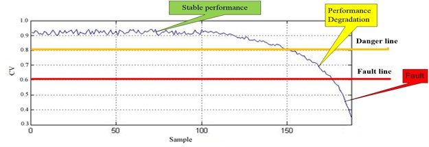
As $CV$ drops below the predetermined threshold, fault occurs. The CVs of the whole life of tool can be divided into three stages as Fig. 1.

Fig. 1Different stages of CVs during the whole life cycle of tool

2.6. Flow of the proposed method

The aforementioned methods consist of the health assessment process, as depicted in Fig. 2. It can be summarized as below.

Fig. 2Process of tool health assessment

The procedure can be divided into three parts:

Feature extraction: The vibration signal of a tool is decomposes into several IMFs and a residue ${\mathrm{r}}_{\mathrm{n}}$ using the EMD. The IMFs $c_1,c_2,\cdots ,c_n$ and $r_n$ are combined to construct an initial feature vector matrix. The SVD is then employed to obtain the singular values of the matrix, thereby forming the feature vector.

Pattern recognition: Prior to the real-time recognition, a Self-organizing mapping (SOM) network is utilized to map the extracted feature vectors into MQE. The Taguchi method is employed to generate the optimized feature vectors that are used to re-train the SOM, and the original MQEs are recalculated.

Health assessment: The obtained MQE is converted into a CV by a predetermined normalization function. Thus, the health state of the tool can be monitored by tracking its CVs curve.

3.1. Experiment setup

The data in this study captures from runs on a milling machine. The cutting speed is set to 826 rev/min; two levels of cut depth are chosen as 0.75 mm and 1.5 mm; two levels of feed rate are taken as 0.25 mm/rev and 0.5 mm/rev which translate into 413 mm/min and 206.5 mm/min. Cast iron is used as the material. The size of the work-piece is 483 mm × 178 mm × 51 mm. In this research, two experiments with cut depth of 1.5 mm feed rate of 0.5 mm/rev, and cut depth of 0.75 mm feed rate of 0.25 mm/rev were chosen as example 1 and 2.

Fig. 3Sensor mounting position

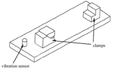
A vibration sensor is mounted on the clamping device on the table, an accelerometer (model 7201-50, ENDEVCO) with a frequency range up to 13 KHz. Its signal is fed into an ENDEVCO 104 charge amplifier with sensitivity 5.71 and 100 mV/g output. The signal is then fed into an ITHACO 4302 Dual 24 dB octave filter with corner frequencies 400 Hz and 1 KHz. The signal is then fed through the PHOENIX CONTACT UMK-SE11,25 cable connector into the high speed data acquisition board of the computer.

Fig. 4Measure of flank wear VB

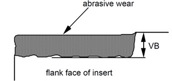
The flank wear VB is measured as the distance from the cutting edge to the end of the abrasive wear on the flank face of the tool. The flank wear was observed during the experiments. The insert was taken out of the tool and the wear was measured with the help of a microscope.

3.2. Experiment results and discussion

3.2.1. Feature extraction

Tool original signal which is nonlinear and non-stationary is shown in Fig. 5. Here, EMD is employed to decompose it into IMFs.

Fig. 5A sample of EMD decomposition results of tool signal

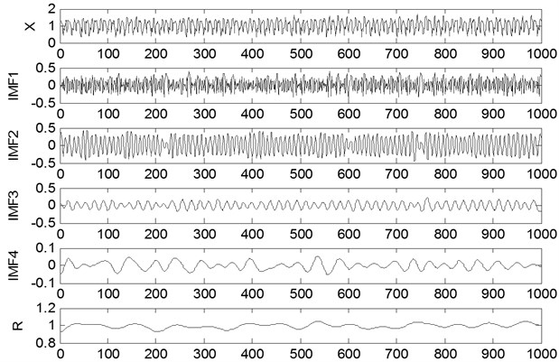
Table 2Feature vector

No.	$E_1$	$E_2$	$E_3$	$E_4$	$E_5$	$R$	$K$	$P$
1	0.4744	0.8642	0.1675	0.0049	0.0109	0.9012	0.7393	0.8068
2	0.4332	0.8964	0.0881	0.0329	0.0040	0.9491	0.7095	0.7624
3	0.4828	0.8629	0.1491	0.0102	0.0041	0.9568	0.7655	0.8175
4	0.5072	0.8504	0.1377	0.0233	0.0069	0.9341	0.7209	0.7720
5	0.4323	0.8862	0.1665	0.0064	0.0067	0.9151	0.7492	0.8014
6	0.4511	0.8832	0.1270	0.0161	0.0080	0.8899	0.7602	0.8130
7	0.5661	0.7986	0.2037	0.0135	0.0027	0.9064	0.7711	0.8280
8	0.4645	0.8684	0.1733	0.0093	0.0038	0.9386	0.7630	0.8181

According to the previous experiences, the first four IMFs which contain the most important information of the signal and a residual error are selected to form a feature matrix, SVD is employed to extract the feature. Then RMS, kurtosis and peak value are added to the feature vector. Table 1 shows 8 groups of normalized feature vectors from the tool with mild wear.

3.2.3. Health assessment

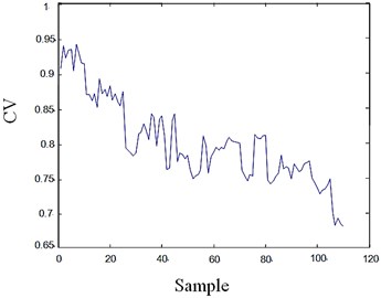
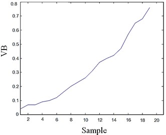
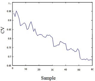
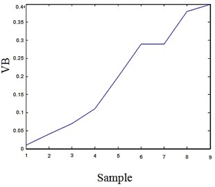
Here 110 samples from example 1 and 60 samples from example 2 are chosen to assess, every five samples are in the same VB. The CV and VB of each group are shown in Fig. 6 and 7.

Fig. 6CV and VB of the tools in example 1

a)

b)

The blue curve in the left Figure shows trend of CV, the first ten samples with CVs above 9.0 indicate the tool is in good state, as the tool operating, CV falls at the same time, but it is still in the range of healthy state, as soon as the CV drop below a given threshold, quality of the work-piece will be influenced at high probability. VB is a index which directly represents the wear of tools. The trend of VB, expressed by the curve in the right Figure, clearly demonstrates that the tool health degenerates tracking as the CV.

Fig. 7CV and VB of the tools in example 2

a)

b)

Example 2, as an assist group, shows the familiar trend with example 1, the VB curve proves the property of the result as well.

Thus it is clear that CV coincidently represents the health of tool and it is also distinctly proved that this approach to health assessment for tools is feasible.