Abstract
The research explores the influence of sampling frequency on the amplitude analysis error for signals with diverse functional forms, and delineates the approach for ascertaining the optimal sampling frequency for amplitude analysis of signals under dynamic monitoring. A method for determining the sampling frequency of amplitude analysis based on the maximum error criterion is proposed through theoretical derivation of sine function and its composite forms. The correctness of the proposed method is further verified through numerical simulation analysis using MATLAB software. The results indicate that the Nyquist sampling criterion does not meet the precision requirements for amplitude analysis; the impact of odd multiples and even multiples `sampling frequencies on the accuracy of signal amplitude analysis is different; the maximum amplitude error is closely related to the order of the signal; and the even multiples sampling frequency is more reasonable for amplitude analysis. The proposed sampling frequency determination method was applied to the construction of dust removal impact testing system and the fatigue damage analysis of a four-section boom pump truck structure, demonstrating the feasibility of this method in engineering applications. The research in this paper provides theoretical and methodological support for the economic collection and efficient processing of massive condition monitoring signals in engineering practice.
1. Introduction
Structural health monitoring (SHM) synthesizes expertise from diverse disciplines, encompassing modern sensor technology, network communication, signal processing, data management, early warning technology and structural analysis, etc. [1]. The dynamic signals of a structure usually contain abundant health status information. By collecting and analyzing these dynamic signals, the safety status, fatigue life, and overall performance of the structure can be monitored and assessed [2-5]. The sampling frequency exerts a pivotal influence not only on the precision of dynamic signal analysis but also on the real-time assessment of structural safety and the forecasting of structural degradation trends. An appropriately selected sampling frequency can diminish the costs associated with monitoring and enhance the efficiency of data processing. Excessive sampling frequencies may lead to a dramatic increase in data volume, imposing higher demands on data acquisition, processing, and storage capabilities of the monitoring system; insufficient sampling frequencies may fail to preserve the critical points of dynamic monitoring signals, resulting in significant discrepancies between monitoring outcomes and actual conditions. Ensuring both the precision of signal analysis and the reliable operation of the monitoring system, the economic collection of dynamic signals has become a critical issue in state monitoring systems.
Common signal sampling methods include up-sampling, down-sampling, under-sampling, etc. [6-8]. Wu [9] focused on the strategy of sampling frequency selection in parameter estimation under unknown time shift stat. Renner [10] determined the effect of sampling frequency on metrics of impact kinetics during landing, walking, and running. Do [11] optimized the sampling frequency for coastal seawater quality based on mathematical models and natural and human activities. Hua [12] analyzed the impact of sampling frequency on the time-domain signal amplitude, and determined the maximum sampling frequency limit of undistorted signals, thereby providing reference for the determination of the sampling frequency for the real-time monitoring of the deflection of small-and medium-span bridges. Romagnoli [13] originally sampled at 4 Hz, then resampled at 2 Hz, 1 Hz, 0.4 Hz and 0.2 Hz, and automatically analyzed using CTG Analyzer. The results obtained through automatic analysis were compared with visual labeling to obtain the optimal sampling frequency. Xiao [14] down-sampled the signals with frequencies ranging from 1 Hz to 500 Hz to examine the discrepancies between the original signals and the down-sampled ones, and the minimum sampling frequency is derived from the results of the study. Saatci [15]derived the constraint conditions for sampling frequency using the geometric method of bandpass sampling theorem. This unified structure directly links the geometric method of bandpass sampling theorem with optimization problems, and verifies the effectiveness of this method in terms of minimum sampling frequency and computational efficiency through numerical simulation. Zhuo [16] proposed and evaluated a compressed sensing AE signal acquisition system. Li [17] proposed a new wavelet based spatiotemporal sparse quaternion dictionary learning (WSTS-QDL) algorithm for reconstruction of multi-channel vibration data. Ji [18] proposed a phased array image method based on compressive sampling and data fusion for wireless structural damage monitoring. Liang [19] chose the random demodulation system is to realize compressive sensing, and the corresponding hardware and software systems were designed, to compress and sample signal and reduce the sampling rate and the amount of data at the same time.
In this paper, the impact of sampling frequency on amplitude analysis error is explored on sine function and its composite forms. A general formula for determining the sampling frequency based on the maximum error criterion was proposed. Furthermore, the method was applied to the structural health monitoring of a four-arm concrete pump truck and the construction of a dust removal impact testing system, and its feasibility has been verified.
2. Generalized sampling theorem
Discrete signals are usually obtained by sampling continuous signals, which only reflect partial information of the original signal. The selection of sampling frequency is related to the purpose and accuracy of signal analysis. Frequency domain analysis in engineering generally follows the Nyquist sampling theorem: the sampling frequency fs must be greater than or equal to twice the highest frequency f0in the signal, as shown in Eq. (1) [20]:
To facilitate computer processing, Eq. (2) is generally used:
In practical engineering applications, in order to ensure the accurate capture of the frequency components of the original signal and avoid frequency aliasing, considering that the filter cannot have ideal cutoff characteristics and there is a certain range of transition bands after the cut-off frequency f0, generally Eq. (3) is used:
The above sampling criteria are based on the aliasing problem in frequency domain analysis, without considering the impact of sampling frequency on the accuracy of time domain analysis. As shown in Fig. 1(a)-(d), sine signal with natural frequency of 2 Hz is sampled at sampling rates of 2 times, 2.56 times, 3 times, and 4 times (4 Hz, 5.12 Hz, 6 Hz, and 8 Hz), and triggered at zero time, Fig. 1(a) is sampled at 2 times the fundamental frequency, and the peak and valley values of the sampled signal are both zero; Fig. 1(b) shows a sampling rate of 2.56 times (5.12 Hz), with a peak value of 0.8819 and a valley value of -0.9808; Fig. 1(c) shows a 3 times (6 Hz) sampling rate with a peak value of 0.8660 and a valley value of –0.8660; Fig. 1(d) shows a 4 times (8 Hz) sampling rate with a peak value of 1 and a valley value of –1. The results indicate that the sampled signals can only partially restore the original signal information, and the higher the sampling frequency, the more complete the reconstruction of the original information. Therefore, the Nyquist sampling theorem is the most basic condition to avoid aliasing in the frequency domain. The examples shown in Fig. 1 illustrate that the Nyquist sampling theorem is difficult to meet the requirements of time-domain analysis.
Fig. 1Example of signal sampling lack fidelity
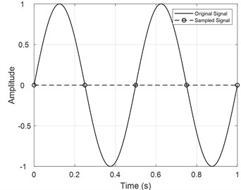
a) 4 Hz
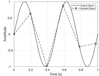
b) 5.12 Hz
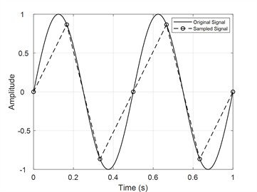
c) 6 Hz
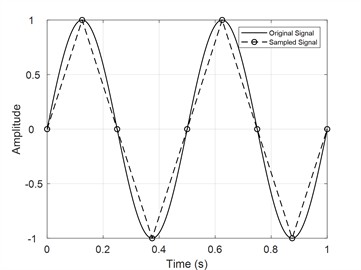
d) 8 Hz
3. Sampling criterion of maximum amplitude error
Spectrum analysis mainly characterizes the overall frequency domain information of signals, but it is difficult to express the subtle characteristics. Many signal analyses are based on time-domain features. For example, the structural alternating stress used for fatigue damage analysis is a typical sine signal, and structural fatigue damage is the logarithm of the amplitude of the alternating stress. The larger the amplitude of the alternating stress, the greater the structural damage caused by each alternating cycle. Therefore, studying the sampling criteria for amplitude analysis is of great significance for the design and operation of condition monitoring systems based on time-domain signal analysis.
3.1. Sinusoidal signal
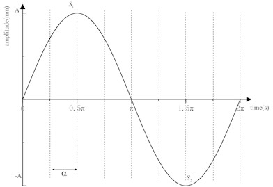
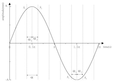
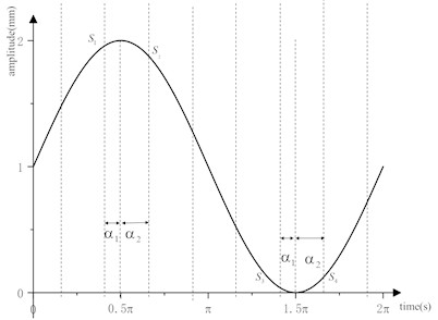
As shown in Fig. 2(a), the frequency of the sine signal is f0 and the amplitude is A. If the sampling frequency is fs, λ is the sampling frequency ratio, and the phase angle between two adjacent sampling points is α (where α=2πλ). For the sinusoidal signal in Fig. 2(a), the most ideal sampling scheme is: when the sampling frequency fs is an even multiple of the original signal frequency f0, the peaks and valleys of the sinusoidal signal can be precisely captured and the amplitude of the discrete signal obtained after sampling has zero error compared to the amplitude of the continuous signal before sampling.
In engineering, the phase relationship between the sampling trigger time and the original signal is usually random, so it is difficult to simultaneously collect the peak and valley points. As shown in Fig. 2(b), whereα1+α2=α, α is the phase difference between two consecutive sampling points, α1 is the phase difference between the peak point and the previous sampling point, α2 is the phase difference between the peak point and the subsequent sampling point.
Fig. 2Schematic diagram of even sampling ratio
a) Example of optimal sampling
b) Example of general sampling
1) If α1<α2, the maximum value after sampling is Smax=S1=Acos(α1), the minimum value is Smin=S3=-S1=-Acos(α1).
2) If α1>α2, the maximum value after sampling is Smax=S2=Acos(α2), the minimum value is Smin=S4=-S2=-Acos(α2).
3) If α1=α2=α/2, the maximum value after sampling is Smax=Acos(α/2), the minimum value is Smin=-Acos(α/2).
The above analysis indicates that different sampling strategies will result in different maximum and minimum sampling values. Due to the randomness of sampling, the most conservative method is to determine the sampling frequency based on the maximum sampling error criterion.
The theoretical derivation approach is as follows: let β=min(α1,α2), then β∈(0,πλ), the maximum value after sampling is Smax=Acos(β), and the minimum value is Smin=-Acos(β). The amplitude relative error after sampling is:
Eq. (4) is an increasing function between 0 and πλ. When the sampling frequency ratio is an even multiple, the maximum error of sampling amplitude can be derived from Eq. (4) as follows:
The minimum error of sampling amplitude is:
According to Eq. (5), as λ increases, the maximum amplitude error rapidly decreases; When λ=2, then δAmax=1, indicating that the Nyquist sampling frequency cannot meet the analysis requirements based on time-domain features. Therefore, signal analysis based on amplitude characteristic parameters requires higher sampling frequency than that signal analysis based on frequency spectrum.
3.2. Composite functions of sinusoidal signals
Complex engineering systems generally exhibit nonlinear characteristics and are subject to the coupling effects of multiple dynamic factors during their operation. Exploring the relationship between the sampling frequency and error of the composite function of sine signals is of great significance.
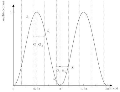
3.2.1. fx=sinnx
For this function, the derivation method for the maximum amplitude sampling error is the same as the sine signal in Section 3.1. Considering the case where n is an even number, the signal period is π and the amplitude is A/2. For instance, n= 2, then fx=sin2x. The curve of this function is shown in Fig. 3(a). If the sampling frequency is fs, λ is the sampling frequency ratio, and the phase angle between two adjacent sampling points is α.
According to the derivation method of Eq. (5), the maximum sampling amplitude error can be obtained as:
The minimum error of sampling amplitude is:
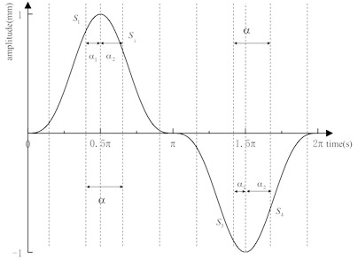
For fx=Asinnx, the detailed reasoning process is as follows: If n is odd, then the signal period is 2π and the amplitude is A. If n=3, the form of the composite function is fx=sin3x, the corresponding curve is shown in Fig. 3(b). According to the derivation method of Eq. (5), the maximum sampling amplitude error can be obtained as:
3.2.2. f(x)=Asin(x)+B
For f(x)=Asin(x)+B, the signal period is 2π and the amplitude is A. If a=1, b=1, then f(x)=1+sin(x), the corresponding curve is shown in the Fig. 3(c), the maximum sampling amplitude error can be deduced as:
Fig. 3Sampling schematic
a)sin2x
b)sin3x
c)1+sinx
4. Numerical simulation
4.1. Sinusoidal signal
At odd sampling frequency ratio, it is impossible to simultaneously collect the maximum and minimum values of the sinusoidal signal, so deriving the relationship between the sampling frequency ratio and the maximum amplitude error using theoretical methods is difficult. Therefore, numerical simulation methods are selected for exploration.
For the sinusoidal signal described in Section 3.1. The numerical simulation approach is as follows: 1) Change the phase difference between the signal occurrence time and the sampling trigger time within the range of 0 to α. 2) Sample the original signal under each phase difference condition, and then extract the sampled amplitude. 3) As the phase difference gradually increases from 0 to α, the sampling amplitude will go through optimal sampling and worst sampling. The maximum and minimum errors corresponding to each sampling frequency can be extracted. To ensure the accuracy of simulation analysis, numerical simulations were conducted using MATLAB software and appropriate sampling intervals were set. For sine signals, the relationship between the sampling frequency ratio and the relative error of the sampling amplitude is shown in Fig. 4(a), 4(b):
1) As the sampling frequency ratio increases, the maximum and minimum error curves of the sampling amplitude decrease in a zigzag pattern and tend towards zero.
2) For the maximum error in sampling amplitude, the error corresponding to the even sampling frequency ratio is greater than the error corresponding to the adjacent odd sampling frequency ratio.
3) When the sampling frequency ratio is even multiple, the minimum amplitude error is 0.
4) Odd multiples of sampling frequency ratio are more optimal considering the maximum amplitude error, while even multiples of sampling frequency ratio are more optimal considering the minimum amplitude error.
Fig. 4Numerical solution for amplitude error
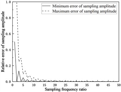
a) Maximum and minimum error of sampling amplitude for sinusoidal signal
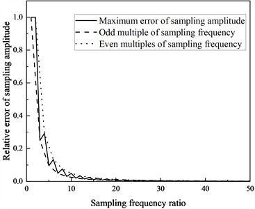
b) Maximum error of sampling amplitude on odd and even multiple sampling frequency for sinusoidal signal
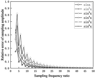
c) Maximum error of sampling amplitude for sinnx
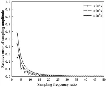
d) Maximum error of sampling amplitude for sinnx (n is even)
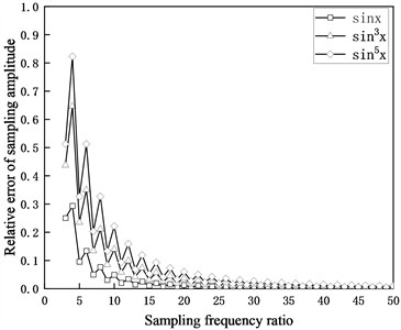
e) Maximum error of sampling amplitude for sinnx (n is odd)
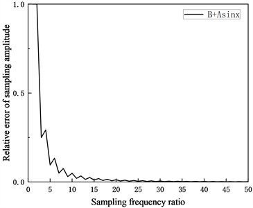
f) Maximum error of sampling amplitude for f(x)=B+Asin(x)
4.2. Sinusoidal complex function signals
For the sinusoidal composite function signal described in Section 3.2. The method of numerical analysis of sine signals in Section 4.1 is also used to explore the composite forms of sine function. The analysis results are shown in Fig. 4(c), 4(d), 4(e), and 4(f):
1) Forsinnx, When n is an odd number, as the sampling frequency ratio increases, the maximum amplitude error curve shows a sawtooth shaped and tends to zero. The higher the signal order, the greater the maximum amplitude error.
2) For sinnx, When n is even, the maximum amplitude error curve shows a decreasing trend, and the higher the signal order, the greater the maximum amplitude error; When only n=2, the maximum amplitude error curve shows a sawtooth shaped decrease and tends towards zero.
3) For f(x)=a+bsin(x), the relationship between the maximum sampling amplitude error and the sampling frequency ratio is the same as that of a sine signal.
In practical engineering applications, it is difficult to accurately control the sampling trigger time and signal generation time, and it is not easy to obtain the amplitude sampling result with the minimum error. Therefore, selecting the sampling frequency based on the maximum error criterion is more in line with engineering practice.
5. Application example
5.1. Sampling frequency for dust removal impact testing system
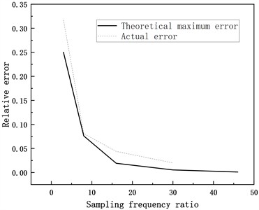
Modal analysis was conducted on the hammer impact system (as shown in Fig. 5), and the first-order natural frequency of the system was 645.67 Hz. During the experiment, the hammer was raised to a 90° position and released to fall freely. When it fell to 0°, the hammer hit the impact bar. The impact signal of force sensor installed on the impact rod was sampled at different fundamental frequency (645 Hz) multiples. The peak value of the impact force at different sampling frequencies is shown in Table 1, and the impact force waveform is shown in Fig. 6. Table 1 and Fig. 6 shows that the peak impact force decreases sharply with decreasing sampling frequency. The actual sampling error and the theoretical maximum sampling error calculated by Eq. (5) are shown in Table 1 and Fig. 7. Table 1 and Fig. 7 shows that the actual sampling error and the theoretical maximum sampling error have the same trend. The actual sampling signal inevitably couples errors caused by other factors, so the actual sampling error is slightly greater than the theoretical sampling error. The project conducted actual testing with a sampling frequency of 10 kHz, and both the theoretical and actual sampling errors were less than 5 %, which is an engineering application of the research results described in this article.
Table 1Comparison between actual sampling error and theoretical sampling error
Sampling frequency ratio | Sampling frequency (kHz) | Sampling peak value (KN) | Theoretical maximum sampling error | Actual sampling error |
46 | 30 | 458 | 0.0011 | – |
30 | 20 | 449 | 0.0055 | 0.02 |
16 | 10 | 438 | 0.0192 | 0.044 |
8 | 5 | 421 | 0.0761 | 0.081 |
3 | 2 | 313 | 0.25 | 0.317 |
Fig. 5Dust removal impact testing system
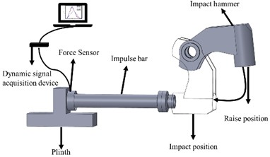
Fig. 6Waveforms at different sampling frequencies
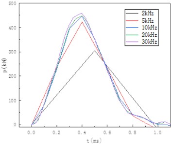
Fig. 7Sampling error trend
5.2. Effect of sampling frequency on the accuracy of fatigue damage analysis
5.2.1. Theoretical analysis of fatigue damage
The fatigue performance of engineering structures is related to the material and structural. The S-N curve is often used to describe the relationship between the alternating stress amplitude of the material and its fatigue life [21]:
where a, b are constants, usually determined by experiments; σi is the fatigue strength, which is the amplitude of the cyclic alternating stress; Nidenotes the corresponding fatigue life.
The damage caused by a stress cycle with an amplitude of Eq. (11) is given as:
If the even-fold sampling frequency ratio is λ, the symmetric cyclic stress amplitude is σa, according to Section 3.1, the stress amplitude corresponding to the maximum amplitude error is:
σS is the sampling result of stress cycle amplitude. By substituting Eq. (13) into Eq. (12), Eq. (14) can be obtained:
Dsis the damage value corresponding to σS. By combining Eq. (12) and (14), the relationship between the maximum damage error and the sampling frequency ratio λ can be obtained:
Simplification of Eq. (15) gives:
5.2.2. Numerical simulation of fatigue damage error
If the S-N curve of the material is:
Carried the parameter b= –3.331 in Eq. (17) into Eq. (16):
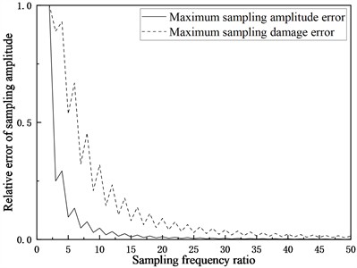
Fig. 8 shows the relationship curve between δD and λ in Eq. (20), and the results indicate that:
1) As the sampling frequency ratio increases, the maximum fatigue damage error δD decreases in a sawtooth pattern and tends to zero.
2) The maximum damage error is greater than the corresponding amplitude error at the same sampling frequency ratio, so the requirement for sampling frequency in damage analysis is higher than that in amplitude analysis.
Fig. 8Damage error versus frequency ratio
5.2.3. Sampling frequency for structural health monitoring of pump truck booms
Taking the four-section arm pump truck in the literature [22] as an example, the proposed sampling frequency determination method is applied to structural health monitoring system. The pumping frequency of the pump truck is 0-0.4 Hz, and the first-order natural frequency of its arm under different deployment postures is 0.39 Hz-0.67 Hz. Therefore, a frequency of 0.67 Hz is taken as the basis for determining the sampling frequency of the health monitoring system.
The stress of the pump truck arm structure consists of two parts: One part is the long time-range stresses caused by quasi-static loads such as changes of the pump truck’s boom posture; One part of the vibration stress is caused by periodic pumping loads, which contains a high frequency component and requires a high sampling frequency. The vibration stresses include the forced response to periodic pumping excitation and the free vibration response to pumping impact, which correspond to the pumping frequency response and the intrinsic frequency of the boom structure, respectively.
The monitoring strain signals of monitoring points 1# and 2# of the pump truck during a certain period of time are shown in Fig. 9. According to the Nyquist sampling theorem, a frequency of 2 Hz satisfies the anti-aliasing requirements. The actual sampling error and theoretical sampling error under different sampling frequencies calculated by Eq. (20) are shown in Table 2 and Table 3. As can be seen from Table 2 and Table 3, the theoretical maximum sampling error corresponding to the Nyquist sampling frequency is 0.8898, and the actual sampling error corresponding to measurement point 2# is 0.1414; when the sampling frequency reaches 20 Hz, the theoretical error is less than 5 %, and when the sampling frequency is 50 Hz, the theoretical error is less than 0.5 %. The actual sampling error is smaller than the theoretical maximum sampling error. Therefore, it is feasible in engineering to determine a sampling frequency of 50 Hz based on the maximum error sampling criterion.
Fig. 9Strain course of monitoring point

a) 1# monitoring point
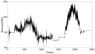
b) 2# monitoring point
Table 2Comparison between actual sampling error and theoretical sampling error for monitoring points 1#
Sampling frequency ratio | Sampling frequency (Hz) | Calculated damage values | Theoretical maximum sampling error | Actual sampling error |
150 | 100 | 1.22E-05 | 0.0017 | – |
75 | 50 | 1.22E-05 | 0.0034 | 0 |
30 | 20 | 1.22E-05 | 0.0412 | 0 |
15 | 10 | 1.22E-05 | 0.0808 | 0 |
8 | 5 | 1.22E-05 | 0.4551 | 0 |
3 | 2 | 1.18E-05 | 0.8898 | 0.0328 |
1.5 | 1 | 9.95E-06 | 1 | 0.1844 |
0.75 | 0.5 | 9.95E-06 | 1 | 0.1844 |
Table 3Comparison between actual sampling error and theoretical sampling error for monitoring points 2#
Sampling frequency ratio | Sampling frequency (Hz) | Calculated damage values | Theoretical maximum sampling error | Actual sampling error |
150 | 100 | 3.96E-05 | 0.0017 | – |
75 | 50 | 3.96E-05 | 0.0034 | 0 |
30 | 20 | 3.96E-05 | 0.0412 | 0 |
15 | 10 | 3.86E-05 | 0.0808 | 0.0253 |
8 | 5 | 3.40E-05 | 0.4551 | 0.1414 |
3 | 2 | 3.40E-05 | 0.8898 | 0.1414 |
1.5 | 1 | 1.82E-05 | 1 | 0.5400 |
0.75 | 0.5 | 1.55E-05 | 1 | 0.6161 |
6. Conclusions
1) The Nyquist sampling theorem is mainly applied to frequency-domain analysis, which is the most basic condition to avoid signal aliasing distortion. The Nyquist sampling theorem is difficult to meet the accuracy requirements of time-domain signal analysis. The requirement for sampling frequency in amplitude analysis of dynamic signals is higher than that in spectrum analysis, and the requirement for sampling frequency in structural damage analysis is higher than that in amplitude analysis.
2) For amplitude and damage analysis, the odd and even multiples of sampling frequency have different impact on analysis accuracy, and it is more reasonable to use even multiples of sampling frequency to control the maximum error. For the composite forms of a sinusoidal function, the higher the order of the dynamic signal, the higher the sampling frequency required for amplitude analysis.
3) The sampling frequency determination method based on the maximum error criterion is applied to the health monitoring of a four-arm concrete pump truck and the dust removal impact testing system, verified the feasibility of the proposed method. The method proposed in this paper provides a theoretical basis for the controllable precision acquisition and efficient processing of complex dynamic signals in engineering applications.
References
-
Y. Bao, Z. Chen, S. Wei, Y. Xu, Z. Tang, and H. Li, “The state of the art of data science and engineering in structural health monitoring,” Engineering, Vol. 5, No. 2, pp. 234–242, Apr. 2019, https://doi.org/10.1016/j.eng.2018.11.027
-
N. Eleftheroglou and T. Loutas, “Fatigue damage diagnostics and prognostics of composites utilizing structural health monitoring data and stochastic processes,” Structural Health Monitoring, Vol. 15, No. 4, pp. 473–488, Aug. 2016, https://doi.org/10.1177/1475921716646579
-
L. Peng et al., “Dynamic strain signal monitoring and calibration with neural network based on hierarchical orthogonal artificial bee colony,” Computer Communications, Vol. 159, pp. 279–288, Jun. 2020, https://doi.org/10.1016/j.comcom.2020.05.028
-
T. Singh and S. Sehgal, “Structural health monitoring of composite materials,” Archives of Computational Methods in Engineering, Vol. 29, No. 4, pp. 1997–2017, Oct. 2021, https://doi.org/10.1007/s11831-021-09666-8
-
X.-W. Ye, Y.-H. Su, and P.-S. Xi, “Statistical analysis of stress signals from bridge monitoring by FBG system,” Sensors, Vol. 18, No. 2, p. 491, Feb. 2018, https://doi.org/10.3390/s18020491
-
Q. Jin and Y. Hong, “Self-coherent OFDM with undersampling downconversion for wireless communications,” IEEE Transactions on Wireless Communications, Vol. 15, No. 10, pp. 6979–6991, Oct. 2016, https://doi.org/10.1109/twc.2016.2594176
-
A. Tank, E. B. Fox, and A. Shojaie, “Identifiability and estimation of structural vector autoregressive models for subsampled and mixed-frequency time series,” Biometrika, Vol. 106, No. 2, pp. 433–452, Jun. 2019, https://doi.org/10.1093/biomet/asz007
-
T. Tsubokawa, H. Tajima, Y. Maeda, and N. Fukushima, “Local look-up table upsampling for accelerating image processing,” Multimedia Tools and Applications, Vol. 83, No. 9, pp. 26131–26158, Aug. 2023, https://doi.org/10.1007/s11042-023-16405-7
-
H. Wu, Y. Cheng, and H. Wang, “Modified CRLB based optimal sampling frequency selection in phase and frequency estimation,” IEEE Access, Vol. 7, pp. 36879–36887, Jan. 2019, https://doi.org/10.1109/access.2019.2904792
-
K. E. Renner, A. T. Peebles, J. J. Socha, and R. M. Queen, “The impact of sampling frequency on ground reaction force variables,” Journal of Biomechanics, Vol. 135, p. 111034, Apr. 2022, https://doi.org/10.1016/j.jbiomech.2022.111034
-
H. T. Do and L. A. Phan Thi, “Optimization of sampling frequency for coastal seawater quality monitoring,” Environmental Monitoring and Assessment, Vol. 192, No. 11, p. 731, Oct. 2020, https://doi.org/10.1007/s10661-020-08700-9
-
W. Hua, R. Wang, J. Hu, H. Li, and X. Sun, “Determination method for conversion sampling frequency of structural deflection monitoring of small-and medium-span bridges,” IOP Conference Series: Materials Science and Engineering, Vol. 794, No. 1, p. 012025, Mar. 2020, https://doi.org/10.1088/1757-899x/794/1/012025
-
S. Romagnoli, A. Sbrollini, L. Burattini, I. Marcantoni, M. Morettini, and L. Burattini, “Digital cardiotocography: What is the optimal sampling frequency?,” Biomedical Signal Processing and Control, Vol. 51, pp. 210–215, May 2019, https://doi.org/10.1016/j.bspc.2019.02.016
-
Z. G. Xiao and C. Menon, “An investigation on the sampling frequency of the upper-limb force myographic signals,” Sensors, Vol. 19, No. 11, p. 2432, May 2019, https://doi.org/10.3390/s19112432
-
E. Saatci and E. Saatci, “Determination of the minimum sampling frequency in bandpass sampling by geometric approach and geometric programming,” Signal, Image and Video Processing, Vol. 12, No. 7, pp. 1319–1327, Apr. 2018, https://doi.org/10.1007/s11760-018-1285-x
-
Z. Pang, M. Yuan, and M. B. Wakin, “A random demodulation architecture for sub-sampling acoustic emission signals in structural health monitoring,” Journal of Sound and Vibration, Vol. 431, pp. 390–404, Sep. 2018, https://doi.org/10.1016/j.jsv.2018.06.021
-
Q. Li, “Wavelet-based spatiotemporal sparse quaternion dictionary learning for reconstruction of multi-channel vibration data,” Applied Soft Computing, Vol. 167, p. 112354, Dec. 2024, https://doi.org/10.1016/j.asoc.2024.112354
-
S. Ji, C. Tan, P. Yang, Y.-J. Sun, D. Fu, and J. Wang, “Compressive sampling and data fusion-based structural damage monitoring in wireless sensor network,” The Journal of Supercomputing, Vol. 74, No. 3, pp. 1108–1131, Dec. 2016, https://doi.org/10.1007/s11227-016-1938-x
-
D. Liang, Q. Han, Y. Cai, K. Yu, and Y. Zhang, “Compressive sampling system based on random demodulation for active and passive structural health monitoring,” Smart Materials and Structures, Vol. 31, No. 6, p. 065005, Jun. 2022, https://doi.org/10.1088/1361-665x/ac6551
-
P. Bardella, I. Carrasquilla García, M. Pozzo, J. Tous-Fajardo, E. Saez de Villareal, and L. Suarez-Arrones, “Optimal sampling frequency in recording of resistance training exercises,” Sports Biomechanics, Vol. 16, No. 1, pp. 102–114, Jan. 2017, https://doi.org/10.1080/14763141.2016.1205652
-
C. Li, Q. Qi, Q. Dong, Y. Yu, and Y. Fan, “Research on fatigue remaining life of structures for a dynamic lifting process of a bridge crane,” Journal of Mechanical Science and Technology, Vol. 37, No. 4, pp. 1789–1801, Apr. 2023, https://doi.org/10.1007/s12206-023-0319-7
-
G. J. Hua, Y. X. Wu, and S. Wang, “Study of concrete pump truck structural health monitoring,” Advanced Materials Research, Vol. 139-141, pp. 2513–2516, Oct. 2010, https://doi.org/10.4028/www.scientific.net/amr.139-141.2513
About this article

This work was supported by National Key Research and Development Program of China (2023YFC3904603), Key Scientific Research Projects of Hunan Provincial Department of Education (21A0353), Natural Science Foundation of Hunan Province (2023JJ50162).
The datasets generated during and/or analyzed during the current study are available from the corresponding author on reasonable request.
Guangjun Hua: investigation, methodology, experiment visualization, writing-original draft. Yong Shi: formal analysis, writing-review and validation. Wenping Tang: validation, writing-review and editing. Chengji Mi: conceptualization, visualization, supervision.
The authors declare that they have no conflict of interest.
