Voiceprint recognition method of transformer based on LBT-ODF and MVN

1. Introduction

Transformers are key components in power systems, and their operating conditions directly affect the safety and stability of the entire power grid. Early detection and diagnosis of transformer faults are crucial for preventing accidents and reducing economic losses. Traditional fault detection methods rely on regular maintenance and manual inspections, which have issues such as long inspection cycles, high costs, and low accuracy. In recent years, with the development of measurement science and technology, fault detection methods based on acoustic signal recognition have become a research hotspot. These methods analyze the acoustic signals of transformers under different operating conditions, enabling rapid and accurate fault identification [1].

For example, Khan et al. proposed a method for acoustic signal detection using multi-channel acoustic sensors [2]. By placing multiple sensors at different positions on the transformer, they achieved multi-angle and multi-directional acoustic signal acquisition, significantly improving the accuracy of fault detection. This method not only captures weak acoustic signals but also enhances the robustness of detection through multi-channel data fusion.

In terms of signal preprocessing, Kim et al. studied various signal preprocessing techniques for transformer acoustic fault detection. They used adaptive filters and spectral subtraction to preprocess the raw audio signals, effectively reducing environmental noise and high-frequency interference, and improving signal quality (Kim et al. [3]). These preprocessing techniques provide a high-quality data foundation for subsequent feature extraction and analysis [4].

The normal signal of the transformer is shown in Fig. 1(a), Fig. 1(b) represents the voiceprint signal of the transformer reactor bolt loosening, and Fig. 1(c) represents the voiceprint signal of the transformer fan aging.

Fig. 1Normal signal and abnormal signal of the transformer

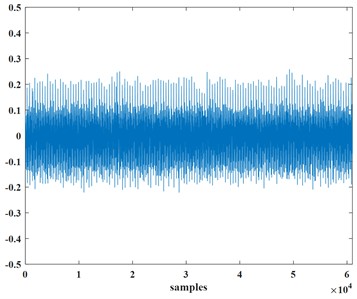
a) The normal signal of the transformer

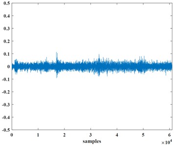
b) Transformer reactor bolt loosening

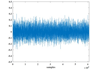
c) Transformer fan aging

Analysis methodoiogies currently employed for transformer vibration signals predominantly feature techniques such as fast Fourier transform, variational mode decomposition [5], and collective empirical mode decomposition [6], Additionally, wavelet packet decomposition and variational mode decomposition methods are also utilized in the analytical repertoire [7, [8], etc. For example, deep convolutional neural networks (DCNN) excel in processing complex vibration signals, effectively extracting features and performing fault diagnosis [9], [10]; long short-term memory networks (LSTM) demonstrate strong capabilities in time series data analysis, capturing long-term dependencies [11], [12]; autoencoders (Autoencoder) are used in unsupervised learning for feature extraction and dimensionality reduction, improving the efficiency and accuracy of signal processing [13], [14]. Compared with the voiceprint method, although the vibration signal identification method has no direct electrical connection with the transformer and has little interference, it requires high detection sensitivity and relies on the installation of the transformer box. The installation location requires further planning [15]. For voiceprint recognition, it is mainly based on traditional time-frequency and other feature information and artificial intelligence perception methods. Literature [16] by collecting the voiceprint or noise signals of dry-type transformers under typical defects such as loose cores and winding deformations for characteristic analysis, the identification of different fault states is achieved. However, the recognition results are susceptible to interference from transformer structure and environmental factors. And proposes a voiceprint recognition method for transformer mechanical faults based on fast incremental support vector data description and gated cycle units. However, the analysis of features is not sufficient. The characteristic values selected by the monitoring system are too single. Neural networks can usually process time series data and mine the connections of data streams on time scales. The literature [17] combines unsupervised learning of stacked autoencoding (SAE) and supervised learning. Combined with the long short-term memory network (LSTM), a transformer diagnosis network framework based on SAE-LSTM is proposed. SAE is used for unsupervised pre-training to remove redundant information. Finally, the SAE training results are sent to the LSTM network for classification. Recognition, literature [18] uses a recurrent neural network architecture (RNN) to capture vibration time series characteristics and use it to determine the possibility of under-excitation, over-excitation and inter-turn faults of early transformers. Generally, convolutional neural networks are suitable for frequency domain information processing of signals. The 1D-CNN network generated by the variant can directly process time series data and feature selection without the need for frequency domain space to avoid excessive calculations and overly complex feature factors. problem, it is more suitable for fault identification of transformer sound signals. Applying LBP and LTP methods to one-dimensional sound signals facilitates the acquisition of crucial data regarding the local temporal features of sound, and at the same time, single features or mixed mining features need to be considered to ensure better recognition accuracy [19], [20].

This paper proposes an innovative network model (LBT-ODF-MVN) that integrates a custom feature space domain, multiple one-dimensional CNN modules, and a multi-channel decision module for the acoustic recognition of transformer mechanical faults. First, we extract local time-domain related features from the one-dimensional signal sequences of fault samples. To compensate for the loss of global information, this study introduces discrete and fitting features, which are embedded into the custom feature space LBT. This custom feature space not only considers the significance of different feature sequences but also captures their internal relationships, thereby better preserving the rich information in the data.

Furthermore, to fully utilize multi-scale information, we construct a Multi-View Network (MVN) model, which further enhances the fault recognition capability. Experimental results show that the proposed LBT-ODF-MVN model exhibits high efficiency and accuracy in fault recognition tasks. Specifically, by combining local time-domain features with multi-scale information, our model can more comprehensively capture fault characteristics, significantly improving recognition performance.

The innovations of this study lie in:

– Custom Feature Space: By embedding discrete and fitting features, we form a unique feature space LBT, which better represents and utilizes the complex information in the data.

– Multi-View Network Model: The MVN model allows us to integrate information from different scales, enhancing the robustness and accuracy of fault recognition.

– Multi-Channel Decision Module: Through the multi-channel decision module, we can effectively utilize the outputs from multiple one-dimensional CNN modules, further improving recognition performance.

These innovations not only advance the technology of acoustic recognition for transformer mechanical faults but also provide important technical support for practical engineering applications.

2. CNN transformer voiceprint recognition based on one-dimensional fusion features

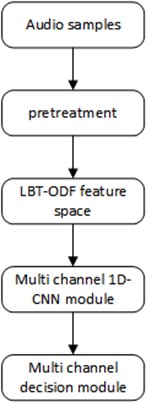
The process of transformer fault voiceprint recognition primarily consists of two main components: feature extraction and algorithmic identification. In this paper, we construct a custom feature space using LBT-ODF features and propose a transformer voiceprint recognition method based on a multi-channel network model. The recognition process is illustrated in Fig. 2. To enhance the efficiency of the overall model, we preprocess the raw audio signals using a fifth-order Butterworth bandpass filter (25-400 Hz) to reduce noise. The filtered signals are then transformed from the time domain to individual feature vectors and mined feature vectors. We use LBT-ODF features to build a custom feature space, which includes Local Binary Patterns (LBP) and Local Ternary Patterns (LTP) to capture local characteristics of the acoustic signals. Additionally, we employ one-dimensional Local Binary Patterns (1D-LBP) and one-dimensional Local Ternary Patterns (1D-LTP) to further refine the feature extraction. The multi-channel one-dimensional CNN structure includes four convolutional layer modules, an attention mechanism module, and a recognition module to process each feature vector. Finally, the designed multi-channel decision module performs a majority voting decision on the classification results obtained from each one-dimensional CNN model, generating the final result.

Fig. 2Voiceprint recognition process

3. Preprocessing

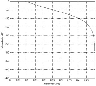
Preprocessing is the fundamental step in our method. As mentioned in [21], this article uses a fifth-order Butterworth filter with a bandpass of 25-400 Hz to reduce noise from the transformer sound signal. For the design of the filter, the 1 dB frequency band is selected through attenuation. Fig. 3 represents the amplitude response, which shows that the response is initially flat and then gradually decreases.

Fig. 3Filter amplitude corresponding

4. LBT-ODF feature space

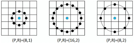
The feature space articulated herein is predominantly crafted from a blend of two categories of amalgamated data, encompassing local feature particulars and self-mined insights. These constitute the Local Binary Pattern features (LBP) and the Local Ternary Pattern information (LTP), respectively. LBP was originally in article [22]. The approach entails partitioning the image into several segments to harvest local characteristics. Typically, LBP is delineated through three distinct circular vicinities. Illustrated in Fig. 4 are the trio of LBP operators, as referenced in [20].

Fig. 4Three domain definitions

Each pixel in the image is bestowed with an LBP label, constituted by a series of 1’s and 0’s. These binary labels are generated through a comparative analysis between each pixel and its surrounding $N$×$N$ neighborhood, centered on the focal pixel. Under the LBP scheme, a pixel is denoted as 1 should its value exceed or match that of the central pixel; conversely, it is flagged as 0 if lesser. A visual representation of pixels coded by the LBP operator can be observed in Fig. 5.

Fig. 5LBP extraction process

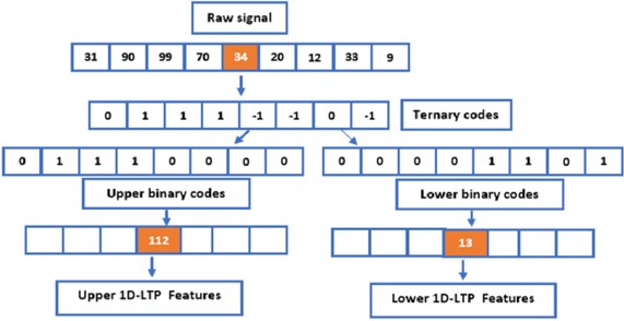
In an unprecedented move, the one-dimensional local binary pattern (1D-LBP) technique was adapted for use with speech signals, taking inspiration from the procedural framework of 2D-LBP in article [17]. The operational sequence mirrors that of its two-dimensional relative. Initially, a predefined number of samples are chosen, and the signal's pivotal point is established; within this work, a sample ensemble of 8 elements is adopted. Adhering to the principles of 2D-LBP, each successive signal value undergoes comparison against the central datum – those exceeding or equating to it receive a binary code of 1, while lesser values are denoted by 0. This comparative analysis is iteratively conducted across the entirety of the signal series. Ultimately, the central signal datum is supplanted by the aggregated, weight-adjusted sum of proximate values, leading to the derivation of a feature vector spanning 1×$N$ dimensions. The binary pattern relationship intrinsic to each signal value manifests thusly:

where $g_c$ is the center of the signal, $P$ is the number of signal sample values in the neighborhood, and $2^P$ is the coefficient of the signal sample value in each neighborhood. Fig. 6(a) delineates the magnitudes of both the neighboring and central samples. In Fig. 6(b), those domain samples surpassing the values of the $P_c$ samples are annotated with a digit of 1, juxtaposed against the rest, which are inscribed as 0. Fig. 6(c) illustrates how the central signal value corresponds to the weighted summation of its surrounding values, referenced in relation to the central sample.

At the same time, rapid energy conversion often brings problems such as insufficient information extraction, and LBP is easily affected by noise and acoustic sample fluctuations [20]. In order to further improve the recognition ability of LBP, this article embeds the LTP feature into the feature vector and converts the signal from the time domain to the custom feature domain. LTP encapsulates the relational dynamics between a pixel and its domain, manifesting as “greater than”, “equal to”, or “less than”. When subjected to identical sampling parameters, LTP yields a richer, more intricate soundscape of features vis-à-vis 1D-LBP. Within the LTP framework, threshold selection adopts a tripartite valuation scheme, contingent upon the interplay between the focal pixel and its neighbors. These values correspond to 0, 1, and –1, respectively, delineating the comparative outcomes.

Fig. 6Extraction steps of 1D-LBP

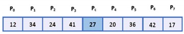
a) Sampled data of sub-signals

b) binary representation of the signal with 8 sample points and center

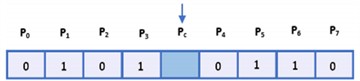
c) binary number representation

The Eq. (2) is usually chosen to calculate LTP characteristics:

where $S\left(X\right)$ represents the ternary mode acoustic signal, $q_i$ represents the domain sample value, $p$ represents the center sample value, and $t$ represents the threshold. The 1D-LTP features are garnered from the signal’s upper and lower segments. These are meticulously computed and encoded, leveraging both lower and upper threshold values, as detailed subsequently Eq. (3a) and Eq. (3b):

Fig. 7LTP feature extraction process

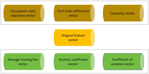
After obtaining three sets of feature vectors of a single sound signal data, in order to mine as much information as possible in the feature sequence, this paper defines three types of features according to the characteristics of feature calculation: original features, discrete features and fitting features. Original features describe the original distribution of data, discrete features mainly describe the degree of dispersion and changing trends between data, and fitting features mainly show the contextual and implicit characteristics of the data.

If the overall LBT sequence is rough, there may be an increasing or decreasing trend locally. This increasing or decreasing trend feature can be extracted through the first-order difference operation: the second-order difference of the sequence can further represent continuous adjacent The change of concavity and convexity between value values; and the occupancy ratio is the proportion of the difference between the current value and the minimum value in the current sequence to the difference between the overall maximum and minimum values, which can make the abnormal data characteristics at the extreme points more obvious because of them They are all obtained by processing data using discrete statistical methods, so this article classifies first-order differences, occupancy ratios and concavity as discrete features. The fitting feature takes the “sliding window” as an opportunity to consider the integrity of the vector and the correlation between time series data, making up for the shortcomings of considering a single sample value in the original features and discrete features [19], so This paper selects kurtosis coefficient, coefficient of variation, and moving average as fitting features [18], [19].

Suppose the original feature vector is $\left(q_1,q_2,\dots ,q_m\right)$, where $m$ denotes the extent of the dataset and $q$ is the value of the $i$-th time point.

(1) Original features.

The original data is defined as the original feature, and the original feature value of the sequence $F=\left(f_1,f_2,\dots ,f_m\right)$ is the same as $\left(q_1,q_2,\dots ,q_m\right)$.

(2) Discrete characteristics.

1) The first-order difference is the difference between consecutive adjacent value values, which can represent the change of local monotonicity between adjacent data. The first-order difference $D=\left(d_1,d_2,\dots ,d_m\right)$ of the sequence is Eq. (4):

2) The occupancy ratio quantifies the ratio of the gap between a feature’s current measurement and the least value within the sequence, juxtaposed with the amplitude spanning from the highest to the lowest value across the board. This ratio is advantageous in highlighting the unique attributes of data points that fall into outlier categories at the boundaries.

3) Concave-convexity represents the change of concavity and convexity between consecutive adjacent values, and is defined by the second-order difference. Concave-convexity is a supplement to the first-order difference:

(3) Fitting features.

The fitting feature is based on the sliding window. Let the data in the sliding window be win and the size of the window be $w$. The vectors are processed using the “delay embedding method”:

1) Kurtosis coefficient:

It describes whether the time series is heavy-tailed or light-tailed relative to the normal distribution, where $E$ represents the mathematical expectation and $w$ represents the size of the sliding window. Time series with high kurtosis tend to have heavier tails or outliers, making them better at detecting sudden spikes or dips.

2) Coefficient of variation:

It describes the dispersion of a sequence in a sliding window, indicates the extent to which the data is concentrated on the average value, and reflects the overall change of a sequence.

3) The average moving line describes the average value of the corresponding sequence in the sliding window. It weakens irregular changes in time series and reveals changing trends among data:

Fig. 8Custom feature space

5. MVN model

After completing the construction of the multi-dimensional feature domain, taking into account the meaning and intrinsic relationship of different feature sequences, in order to fully integrate multi-scale information, this paper constructs an MVN model to complete the fault identification task. The model structure is shown in Fig. 9.

Fig. 9MVN model

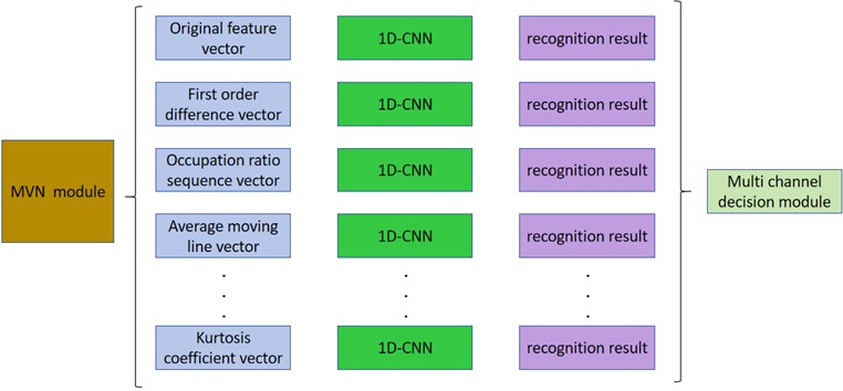
Featuring multi-dimensional feature vectors as its input, the one-dimensional CNN construct is anchored by four convolution sections, an Attention Mechanism (AM) module, alongside a categorization unit delivering early results. Thereafter, a dedicated decision-making segment furnishes the terminal recognition outcomes.

5.1. Convolution module

The one-dimensional convolutional layer [23] uses a one-dimensional filter with a preset width to locally convolute the input data in the order of steps, and then outputs the corresponding result. The calculation method of convolution is Eq. (10):

10

$y_i^l={\sum }_{j=0}^{k-1}{x}_{i+j-bk/2c}^{l-1}\cdot w_j^{l,k}+b^{l,k},$

where $x_i^l$ is the input signal centered on position $i$ of the $l$-th layer, $w_k^{lT}$ and $b_k^l$ are the weight matrix and bias term of the $k$-th filter of the $l$-th layer respectively, and $z_{ik}^l$ is the $k$-th feature map of the $l$-th layer. The kernel sizes for the quartet of convolution modules are standardized at 3, with kernel quantities established at 32, 32, 64, and 64 correspondingly. Given the shared parameter framework, each layer’s convolution kernel count synchronizes with its respective convolutional layer’s feature map quantity. Thus, reduced kernel numbers in superficial layers capture fundamental, lower frequency attributes, and increased kernel counts in more profound layers harvest a plethora of higher frequency features. This approach minimizes parameters, safeguarding against excessive model training on noise. Post-convolution, Batch Normalization (BN) is a pivotal inclusion, expediting training, stabilizing gradients, and regularizing, thereby amplifying convergence rates and network sturdiness. A modified linear unit, acting as the activation function post-BN, bolsters non-linearity. The pooling layer refines extracted information into a condensed, vectorial representation, preserving salience whilst discarding trivialities. Architecturally, it diminishes succeeding layer inputs via subsampling, alleviating computation and endowing shift tolerance. Max pooling, by electing maximal values within regions, following the secondary convolution segment, safeguards textural traits, with its operation defined as Eq. (11):

11

$p_{ik}=\mathrm{m}\mathrm{a}{\mathrm{x}}_{(o,p)\in R_{ik}}\left(y_{koq}\right),$

where $y_{koq}$ is the element at $(o,p)$ in the pooling region $R_{ik}$, representing the local neighborhood near the $k$-th feature map position $i$, $p_{ik}$ is the relevant output after the pooling operation. This article sets the size and stride of the pooling kernel to 2.

Fig. 101D-CNN

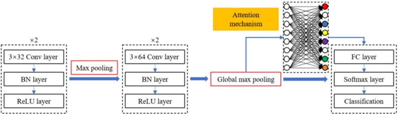
Global max pooling, through its selection of the supreme element across all feature maps, prunes the fully connected layer's parameter set in both the Attention Mechanism and classification modules, proficiently averting overfitting whilst concurrently conserving computational power and time. Consequently, a global max pooling level is instituted post-quartet convolution and pre-AM module:

12

$g_k=max\left(y_k\right).$

Among them, $y_k$ is the activation value of the $k$-th feature map, and $g_k$ is the relevant output of the pooling operation.

6. Experiments and results

The test object of this study is a custom-made real-type oil-immersed converter transformer, model D-800/35. The design parameters and structural characteristics of this transformer allow it to simulate various operating conditions found in actual operation. The experimental setup includes the following main components: the transformer body, acoustic sensors, and sensor placement. The transformer body is a D-800/35 type oil-immersed converter transformer, capable of simulating different mechanical fault scenarios. The acoustic sensors consist of high-performance microphones and high-precision acquisition cards. The frequency response range of the microphones is 3.5-20000 Hz, allowing them to capture a wide range of acoustic signals. The acquisition card model is DP240, with a maximum sampling frequency of 102.4 kHz, ensuring high-resolution and high-precision data. The experimental setup is as shown. To comprehensively capture the acoustic signals at different positions on the transformer, we placed three microphones on the front, side, and diagonal corners of the transformer. Each microphone is positioned at the same height as the center of the transformer and is 0.5 meters away from the transformer’s surface. This multi-point placement provides more comprehensive and accurate acoustic data.

Fig. 11Experimental layout

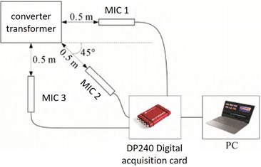
To ensure the accuracy and reliability of the experimental data, we adopted the following data collection methods: First, the sampling frequency was set to the maximum sampling rate of 102.4 kHz. A high sampling rate captures more detailed information, enhancing the resolution and accuracy of the data. Second, data collection from all sensors is synchronized to ensure temporal consistency of the acoustic signals from different positions, which aids in subsequent data analysis and fault diagnosis. During the experiment, we strictly controlled the experimental environment to minimize external noise interference. The laboratory was kept quiet, and other machinery was avoided to ensure the purity of the collected acoustic signals. Each experiment lasted 10 minutes, with acoustic signals recorded every minute. During data recording, we used professional data acquisition software to monitor data quality and collection status in real-time, ensuring the integrity and reliability of the data. Finally, the raw data collected were preprocessed, including noise reduction and filtering steps, to reduce the impact of environmental noise and improve signal quality. The preprocessed data were used for subsequent feature extraction and analysis.

A total of 9180s of valid audio were collected. These audios were then classified, labeled, and classified into data sets, and the audios were divided into 6 situations: excitation, current, loose core excitation, loose core current, loose coil excitation, and loose coil current. Within this experimental setup, the proportion of the training dataset to the testing dataset approximates a ratio of 8:2.

To more accurately quantify the uncertainty of the measurements, we used the Standard Error (SE) in the experimental results to assess the stability of the measurement outcomes. The standard error measures the standard deviation of the sample mean, reflecting the variability of the sample mean. A smaller standard error indicates a more precise estimate of the sample mean and more stable measurement results. The formula for calculating the standard error is shown Eq. (15):

where $s$ is the sample standard deviation, $n$ is the sample size.

The confidence interval (CI) provides a range within which the true population mean is likely to fall. A 95 % confidence interval means that we are 95 % confident that the true population mean lies within this interval. The narrower the confidence interval, the less uncertainty there is about the measurement results:

where $\stackrel{-}{x}$ is the sample mean, $t_{\alpha /2,n-1}$ is the critical value of the $t$-distribution, $s$ is the sample standard deviation, and $n$ is the sample size.

The coefficient of variation (CV) is used to measure the relative variability of the data. It is calculated as the standard deviation divided by the mean, expressed as a percentage. A smaller coefficient of variation indicates lower relative variability and more consistent measurement results:

The standard errors for the measurement results of excitation fault, current fault, core loosening excitation fault, core loosening current fault, coil loosening excitation fault, and coil loosening current fault are 0.028, 0.021, 0.017, 0.012, 0.016, and 0.024, respectively.

The 95 % confidence intervals for the measurement results of excitation fault, current fault, loose core excitation fault, loose core current fault, loose coil excitation fault, and loose coil current fault are 0.94, 0.98, 0.97, 0.93, and 0.92, respectively.

The coefficients of variation (CV) for the measurement results of excitation fault, current fault, loose core excitation fault, loose core current fault, loose coil excitation fault, and loose coil current fault are 0.051, 0.047, 0.023, 0.042, and 0.036, respectively.

It can be seen that the measurement errors are extremely small, fully meeting the experimental requirements.

This paper first evaluates the rationality of the self-defined feature space, and conducts comparative experiments by constructing a multi-channel network and a single-channel 1D-CNN network. In addition, this article selects two traditional machine learning methods: traditional SVM and KNN, as well as the neural network deep learning methods of Piczak-CNN [24] and MixupCNN [23] for comparative experiments.

This paper compares the proposed LBT-ODF-MVN model with traditional machine learning methods, including Support Vector Machine (SVM) and K-Nearest Neighbors (KNN), as well as deep learning methods such as Piczak-CNN [20] and MixupCNN [21].

The LBT-ODF-MVN model proposed in this paper demonstrates significant superiority in transformer voiceprint recognition tasks, achieving an accuracy of 96.07 %. In contrast, traditional Support Vector Machines (SVM) perform well on small-scale datasets but experience a decline in performance when handling large-scale and high-dimensional data, with an accuracy of only 72.7 %. K-Nearest Neighbors (KNN) algorithms, although simple and easy to use, are sensitive to the scale and dimensionality of the data, leading to higher computational complexity, with an accuracy of 78.3 %. Piczak-CNN performs well in environmental sound classification tasks but has room for improvement in specific domain fault recognition tasks, achieving an accuracy of 83.7 %. MixupCNN enhances the model's generalization capability through data augmentation techniques but still has room for improvement in specific domain fault recognition tasks, achieving an accuracy of 92.2 %. One-dimensional Convolutional Neural Networks (1D-CNN) perform well in handling time-series data but require further optimization in feature selection and processing, achieving an accuracy of 93.2% with raw feature sequences and 93.7 % with first-order difference sequences. The LBT-ODF-MVN model, through its custom feature space and multi-channel decision mechanism, is better able to capture and utilize key features in time-series data, thereby significantly improving recognition accuracy and robustness. These characteristics make the LBT-ODF-MVN model excel in transformer voiceprint recognition tasks, clearly outperforming other methods.

The learning rate hits its nadir at the 20th and 80th epochs, spanning an overall training period of 110 epochs. Employing the stochastic gradient descent optimizer with a momentum of 0.9, and utilizing a 10-fold cross-validation technique, the workflow proceeds as follows: Initially, the dataset of 8732 samples is shuffled and subsequently partitioned into nine folds of 875 samples each, and one fold of 857 samples. The mean outcome of the 10-fold cross-validation is a commendable 95.7 %, while the zenith of accuracy for the model is recorded at 96.07 %. A comparative overview delineated in Table 1 underscores the superiority of our proposed model over those put forth by the majority of alternative research endeavors, alongside conventional machine learning methodoiogies.

Focusing on a selection of prototypical experimental outcomes, as illustrated in Table 2, reveals an outstanding capacity to distinguish loose coil faults, achieving a success rate surpassing 95 %. Performance on other fault types appears less impressive. Analysis of the data suggests that audio signals characterized by higher autocorrelation coefficients and Root Mean Square (RMS) values tend to yield superior recognition rates.

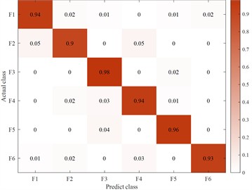
The Fig. 12 describes the training loss curve and category mixing matrix of the LBT-ODF-MVN model. Observe that in the initial 20 epochs, the employment of a larger learning rate instigates persistent oscillations in the loss, which simultaneously undergoes a swift decline. Post the 20th epoch, the model institutes a learning rate reduction, thereby stabilizing and embarking on a quest for the optimal solution.

Fig. 12Training curves of accuracy and loss of the proposed LBT-MVN on the transformer dataset

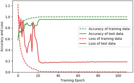
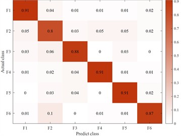
Fig. 13Mixing matrix

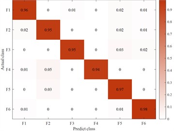
Fig. 14Fuzzy matrix for recognition of different feature inputs in a single channel

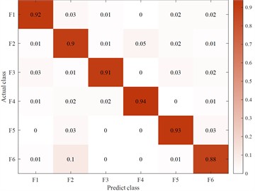
a) Original feature input

b) Occupancy ratio feature input

c) First-order difference feature input

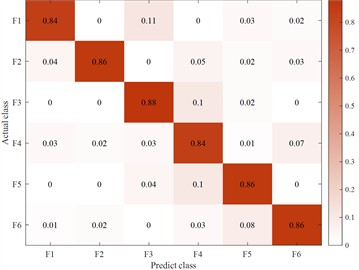
d) Concave-convexity feature input

In order to verify the LBT-ODF-MVN model in this article when the votes are consistent in the multi-channel decision-making module, this article sets the first-order difference sequence as the final recognition result. On the basis of a single channel and excluding the decision-making module, the following conclusions are drawn by comparing the recognition accuracy of each feature sequence. Since the fitting features play a complementary role in the overall local information and have less impact on the subsequent final judgment, this article selects the original features. and discrete feature sequences as single-channel model inputs. By comparing the first-order difference features, the output results are more accurate and meet the setting requirements.

7. Conclusions

This paper proposes a network model (LBT-ODF-MVN) that contains a custom feature space domain, multiple one-dimensional CNN modules and a multi-channel decision module for voiceprint recognition of transformer mechanical faults. First, local time-domain related features are extracted from the one-dimensional signal sequence of the fault sample. In order to make up for the global lost hidden information, this paper embeds discrete features and fitting features to form a custom feature space LBT, taking into account the meaning and meaning of different feature sequences. Internal relationship, in order to fully integrate multi-scale information, this paper constructs an MVN model to complete the fault identification task. The results show the efficiency and accuracy of this article's model and custom feature domain. In future work, other newly proposed and improved 1D-CNN models will be considered to integrate into the overall framework to obtain better recognition methods.