3D GPR profile analysis of interlayer bonding failure in asphalt pavement based on FDTD

Li, Y. X.; Chen, F.; Fu, C. J.; Sheng, S. M.; Kang, X. T.

doi:10.21595/jme.2025.24466

Journal of Measurements in Engineering

Browse Journal

Submit article

Published: 27 February 2025

Check for updates

3D GPR profile analysis of interlayer bonding failure in asphalt pavement based on FDTD

Y. X. Li¹

F. Chen²

C. J. Fu³

S. M. Sheng⁴

X. T. Kang⁵

^{1, 2, 4}School of Energy and Traffic Engineering, Inner Mongolia Agricultural University, Hohhot, China

³Inner Mongolia Jiaoke Road and Bridge Construction Co., Hohhot, China

⁵Hainan Tropical Ocean University, Sanya, China

Corresponding Author:

Y. X. Li

Cite the article Download PDF

Article in Press

Downloads 36

Abstract

Interlayer bonding failure in asphalt pavements, once it occurs, is difficult to detect and address in a timely manner, significantly affecting the road’s lifespan. Three-dimensional ground penetrating radar (GPR) technology can effectively detect internal pavement defects, making it a valuable method for identifying interlayer bonding failure. In this study, the finite-difference time-domain (FDTD) method, implemented using the gprMax software, was employed to establish forward modeling. MATLAB was then used to analyze radar response characteristics under various conditions, including different defect sizes, layer positions, and moisture content levels, after performing 3D reconstruction. Additionally, GPR data were collected from interlayer bonding failures embedded in the field, and the results were compared with numerical simulations to establish the 3D radar profile for interlayer bonding failure in asphalt pavements. These findings were further validated through engineering applications. The results indicate that interlayer bonding failure in the radar profile manifests as discontinuities in the in-phase axis, with a slight “downward-bending” reflection pattern in the B-scan direction. In the direction perpendicular to the B-scan, a “strip” pattern appears, and in the top-down view, a “plate” pattern is observed. An increase in moisture content leads to stronger reflection signals. A moisture content range of 5 %-15 % provides a balanced detection effect, enabling clear identification of the defect area while minimizing interference from overly complex reflection signals. However, when the moisture content exceeds 25 %, the signals become more complex, requiring advanced signal processing techniques to avoid misinterpretation, which may hinder accurate defect identification.

1. Introduction

Interlayer bonding issues refer to the insufficient bonding strength between layers of asphalt pavement, resulting in weak interlayer connections. Most roads in China adopt a semi-rigid pavement structure, and interlayer bonding issues are relatively common in practice. Factors such as material selection, construction quality control, and construction environment can all affect the interlayer bonding condition during construction [1]. The current well-established detection method involves laboratory shear tests to evaluate interlayer bonding strength. Although suitable for quantitative evaluation in laboratory settings, it cannot be used for large-scale field testing. Pull-out tests are also utilized to measure the bonding strength between structural layers, which are applicable to laboratory or small-scale localized areas. While such methods can quantitatively assess interlayer bonding strength, they cannot cover large pavement areas and are destructive [2]-[3]. Although non-destructive radar detection technology has been applied to pavement defect detection, the technology remains immature. The radar characteristic map for interlayer bonding issues is still unclear, making it challenging to quickly and accurately identify interlayer bonding problems. If interlayer bonding issues are not promptly repaired, they can accelerate pavement damage, reduce its service life, and increase maintenance costs [4].

Both domestic and international studies on asphalt pavement interlayer bonding focus primarily on laboratory testing and non-destructive testing technologies. Vaitkus A. et al. [5] assessed the interlayer bonding strength of asphalt layers through direct shear tests (Leutner tests). Wang H. et al. [6] combined theoretical analysis with shear strength measurements to study the interfacial bonding characteristics of flexible pavements and used AASHTO Pavement-ME software to quantitatively analyze the impact of interface debonding on pavement service life. Francesco Canestrari et al. [7] compared the effectiveness of various testing procedures for evaluating interlayer bonding performance of asphalt pavement through laboratory testing. Kai Yang et al. [8] characterized interlayer bonding performance through four parameters: shear strength, tensile strength, flexural strength, and interfacial stiffness. Giri J. P. et al. [9] evaluated the interlayer bonding strength between two common types of asphalt pavement stone layers through laboratory methods. Shang Difei et al. [10] measured the dynamic stability of asphalt mixtures under different bonding conditions and used dynamic stability to evaluate interlayer bonding performance. Kraym, H. M. et al. [11] employed shear tests to validate interlayer bonding strength and analyzed the debonding state of multilayer asphalt pavements.

From the aforementioned research, most studies focus on laboratory testing to assess the interlayer bonding condition of asphalt pavement. These methods are inefficient for detection and cannot effectively and quickly conduct on-site testing. Due to its ability to provide high-resolution images, suitability for rapid detection of large pavement areas, and capability to probe deeper structures, GPR (Ground Penetrating Radar) has increasing potential in road detection applications. In terms of non-destructive testing, L. Zou et al. [12] investigated the capability of a multi-static GPR system to detect delamination between pavement layers using transverse waves, demonstrating the potential of GPR technology in complex pavement structures. P. Shangguan et al. [13] simulated the sensitivity of GPR signals to asphalt pavement density and moisture using the finite-difference time-domain (FDTD) method, providing a calibration method for precise analysis of GPR signals. Dérobert, X. et al. [14] used accelerated pavement testing experiments to monitor artificially delaminated pavement structures with GPR technology. Jiangang Yang et al. [15] analyzed the electromagnetic wave transmission mechanism and its effectiveness in interlayer bonding evaluation through forward modeling and image processing techniques, validating the feasibility of the method. These studies make the application of 3D GPR technology in detecting interlayer bonding issues in pavements increasingly viable.

This paper aims to detect and analyze interlayer bonding issues in asphalt pavements using 3D-GPR technology. Through FDTD numerical simulation and MATLAB-based 3D visualization reconstruction, it explores and proposes radar characteristic maps for interlayer bonding issues in asphalt pavement. The findings provide theoretical support for the rapid diagnosis of interlayer bonding defects using radar technology in the future.

2. Experimental methods

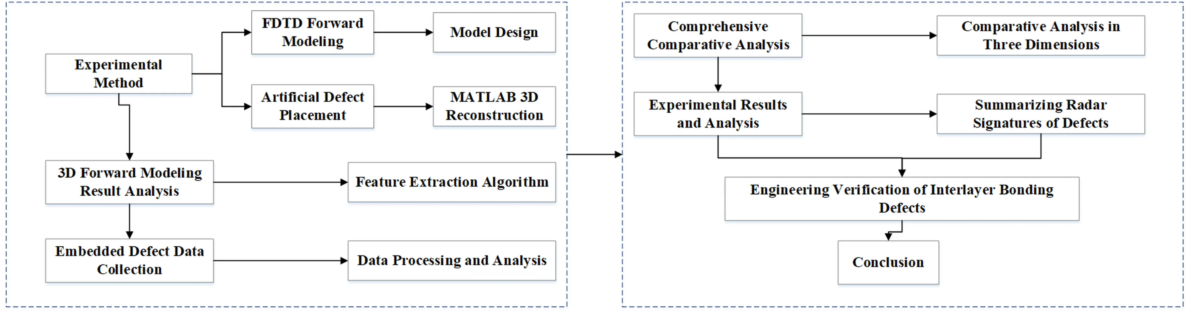
First, based on the analysis of existing literature [16]-[17], two primary locations where interlayer bonding failure commonly occurs were identified. Next, a forward modeling approach using the Finite Difference Time Domain (FDTD) method was employed, and artificial defects were embedded on-site. Three-dimensional ground penetrating radar (GPR) was then used to collect data on the embedded interlayer bonding failures. By comparing the experimental results, the 3D radar characteristic profiles were established. Finally, relying on the project engineering, core sampling was conducted at the locations identified by the radar characteristic profiles to verify the accuracy of the radar signatures of interlayer bonding failure.

2.1. FDTD forward simulation methodology

2.1.1. Forward simulation process

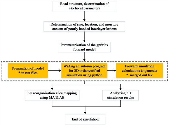
GprMax is a 3D ground penetrating radar (GPR) forward simulation software based on the Finite Difference Time Domain (FDTD) method. It is primarily used to simulate the propagation of electromagnetic waves in isotropic homogeneous media and their interaction with target objects. Users can perform simulations by writing input files for the simulation model (saved as *.in files) and specifying the file path for the input. After the numerical calculations are completed by the computer, the software outputs the B-scan GPR forward simulation results for the target, which are then processed using MATLAB to perform 3D reconstruction, generating 3D volumetric data and forward simulation images. The simulation process of the software is shown in Fig. 1.

Fig. 1gprMax modeling flowchart

2.1.2. Forward model design

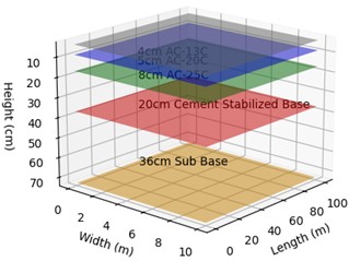
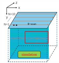
The typical pavement distress site used in this study is a newly paved section. The surface layer consists of 4 cm of AC-13C, 5 cm of AC-20C, and 8 cm of AC-25C; the base layer is made of 20 cm of cement-stabilized crushed stone, and the sub-base layer is 36 cm of low-dose cement-stabilized crushed stone. The construction of the asphalt pavement structure followed the corresponding specifications based on on-site conditions, as shown in the pavement structure schematic diagram (Fig. 2).

For the experimental objectives, the model parameters were designed as shown in Table 1. Considering that the artificially induced interlayer bonding failure is composed of windblown sand and water, the model was designed using the built-in material commands #soil_peplinski and #fractal_box in GprMax software, which can simulate a moisture content up to 25 %. This approach improves the accuracy and fidelity of the model simulation [18].

To balance computational efficiency and model effectiveness, the domain size #domain was set to 2.0×0.9×1.0 meters, and the grid resolution #dx_dy_dz was set to 0.005×0.005×0.005 meters. The time window #time_window was set to 20 ns, corresponding to a depth of 1.0 m, which meets the simulation requirements.

For the actual road detection process, a step-frequency radar system (Norway, 3D-Radar) was used. This equipment is a multi-channel GPR system, and its emitted electromagnetic pulse shape is the same as that of a Ricker wavelet. Therefore, the waveform type #waveform was defined as Ricker. During the modeling process, the model was always within a bounded domain. To prevent the electromagnetic wave from reflecting at the domain boundaries, the boundary absorption condition #pml_cells was set to 10×10×10 cells.

Fig. 2Schematic diagram of the spatial location of the disease and the direction of the survey line

a) Road structures

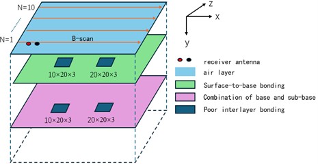
b) Modeling schematic

Table 1Model design parameters

Parameter item	Parameter setting
# domain	2.0×0.9×1.0
#dx_dy_dz	0.005×0.005×0.005
# time_window	20ns
Equipment type	Stepping frequency radar detection vehicle (Norway, 3D-Radar)
Equipment components	GeoScope TM Fourth Generation Radar Host, Antenna Array, Computer, GPS
Number of antennas	10 pairs
# waveform	Ricker
#pml_cells	10×10×10 - 10×10×10
Antenna spacing	2 cm
#src_steps / rx_steps	2 cm
A-scan Channels	65 channels
Simulated antenna pairs	10 pairs

In the GprMax modeling and radar data processing, the relative permittivity is a key parameter for characterizing radar information. It directly influences the propagation speed of electromagnetic waves in the medium, thereby determining the GPR’s detection depth, resolution, and data accuracy. This study analyzes the relative permittivity information of the materials and, in conjunction with the specific pavement structure in the engineering project, derives the main electrical parameters of the pavement, as shown in Table 2.

Table 2Electrical parameter setting information

Asphalt road surface	Materials	Dielectric constant	Thickness
Air	Air	1.0	17cm
Surface layer	AC-13C	3.0	4cm
	AC-20C	3.2	5cm
	AC-25C	3.4	8cm
Base layer	Base	8.0	20cm
Sub-base layer	Sub-base	15.0	36cm

2.2. Artificial disease field deployment methods

According to references [19]-[20], moisture content is an important factor influencing interlayer bonding, especially during construction, where moisture infiltration often affects the interlayer bonding strength due to changes in humidity and environmental conditions. References [21]-[22] point out that defect size has a significant impact on the structural strength of pavements, with larger defects leading to a sharp decline in structural strength, reflecting poor interlayer bonding caused by construction defects or material heterogeneity. To simulate this issue, the experiment used polyethylene bags to wrap sand, simulating interlayer bonding defects. Polyethylene bags have good barrier properties, effectively simulating the impact of moisture infiltration and humidity accumulation on pavement structures. The water absorption properties of sand represent interlayer bonding issues caused by moisture infiltration or poor construction. Furthermore, the method of wrapping sand in polyethylene bags provides good controllability and reproducibility, allowing precise control over factors such as moisture content and defect size [23].

Table 3Artificial defect fabrication parameter settings

Defect type	Size (cm)	Sand mass (g)	Water added (g)	Moisture content (%)
Fixed moisture content disease	10×20×3	365	18	5
	10×20×3	365	36	10
	10×20×3	365	54	15
	20×20×3	720	36	5
	20×20×3	720	72	10
	20×20×3	720	108	15
Disease information for post-addition water	10×20×3	365	Reserved water channel, sealed with T-shaped PVC pipe	–
Disease information for post-addition water	20×20×3	720	Reserved water channel, sealed with T-shaped PVC pipe	–

When preparing defects with fixed moisture content, wind-blown sand was fully dried, sieved to remove impurities, and then fabricated according to the parameters shown in Table 3. For defects with added water, PVC pipes were used to provide a water inlet according to the defect size, with the specific location shown in Fig. 3. First, three-dimensional radar detection was performed on the defects with fixed moisture content, then water was added to the encapsulated loose sand through the embedded PVC pipe, and radar detection was performed again. This step was used to evaluate the impact of the water-added defects on the pavement structure and compare the changes in defect characteristics under different moisture content conditions.

Four experimental groups were designed to explore the radar signature features of interlayer bonding defects at different layer positions, moisture contents, and sizes. The specific experimental setup is shown in Table 4.

Fig. 3On-site artificial defect fabrication

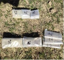
a) Artificial disease models

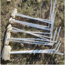
b) T-tube production

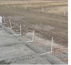
c) Pre-Embedded disease

2.3. Three-dimensional radar data acquisition and processing

To address the issue of indistinct features between the forward simulation data and the measured data, further processing of the raw data is necessary. The specific steps for this process are outlined as follows.

Table 4Experimental design groups

Defect type	Defect location	Size (cm)	Moisture content	Group number
Interlayer bonding defect	Base and sub-base bonding	10×20×3	5 %	Group 1
			10 %
			15 %
			Post-Watering
		20×20×3	5 %	Group 2
			10 %
			15 %
			Post-Watering
	Surface and base bonding	10×20×3	5 %	Group 3
			10 %
			15 %
			Post-Watering
		20×20×3	5 %	Group 4
			10 %
			15 %
			Post-Watering

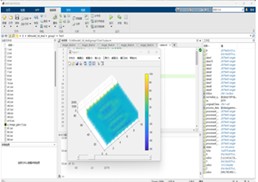
Forward Simulation Data Processing (MATLAB): MATLAB is used to process the forward simulation data, with custom code developed for 3D reconstruction and slicing of the simulated data, resulting in a 3D dataset. This provides an intuitive and reliable data foundation for subsequent analysis. The processing includes:

Reading 2D Data Matrices: The data is read from multiple HDF5 files. After background removal and gain compensation, the amplitude is normalized.

3D Data Matrix Construction: The data is concatenated along the third dimension to form a 3D data matrix (B).

Data Permutation: The data dimensions are adjusted using the permute function, and 3D grid coordinates $X$ , $Y$ , $Z$ are defined.

Slicing for Visualization: The slice function is applied to visualize the 3D data at specified slice positions (xslice, yslice, zslice).

Enhancement of Display: Pseudocolor mapping and smoothing are used to enhance the visual display, with transparency settings adjusted. A slider is included for dynamic adjustment of amplitude, allowing for real-time updates of slice displays for interactive 3D reconstruction and analysis.

Field Data Processing: The data collected from the artificial defects set in the field is processed using Examiner software to ensure the accuracy and completeness of the data. This step facilitates the identification and labeling of defect features in the radar signal.

GPR feature extraction generally involves techniques such as F-K migration processing, image binarization, and Gray Level Co-occurrence Matrix (GLCM). The F-K migration algorithm is employed to reconstruct the actual size and shape of structural defects in the GPR image. The shifted images are then binarized to enhance the display of shape features [24]-[25]. To further enhance the defect features in the horizontal top-down view of the radar data, the Sobel edge detection algorithm is introduced [26]. This algorithm is an effective edge detection technique, known for its high computational efficiency and sensitivity to gradient changes, making it widely applied in edge detection. By calculating the gradients in the $X$ and $Y$ directions, along with the magnitude and direction of the gradient, the Sobel algorithm helps identify key features and boundaries in the radar images.

However, due to the high noise level and complex background of GPR data, direct application of the Sobel algorithm has certain limitations. Specifically, it effectively detects strong reflection interfaces but may miss defects in low-contrast regions. Additionally, it is sensitive to noise, potentially leading to false positives. Therefore, background denoising and gain compensation are performed before feature extraction. The Sobel algorithm is particularly suitable for analyzing material interfaces and defect regions in GPR data [27]-[28].

2.3.1. Sobel algorithm for edge detection

The Sobel algorithm uses two 3×3 convolution kernels (one for the $X$ direction and one for the $Y$ direction) to compute the image gradients in these directions. The gradient reflects the rate of change in pixel intensity, highlighting the edges in the image.

$X$ -direction Gradient ( $G_{x}$ ): This gradient is mainly used to detect vertical edges (horizontal changes).

$Y$ -direction Gradient ( $G_{y}$ ): This gradient is primarily used to detect horizontal edges (vertical changes):

1

$G_{x} = [\begin{matrix} - 1 & 0 & 1 \\ - 2 & 0 & 2 \\ - 1 & 0 & 1 \end{matrix}] * I, G_{y} = [\begin{matrix} - 1 & - 2 & - 1 \\ 0 & 0 & 0 \\ 1 & 2 & 1 \end{matrix}] * I,$

where: $I$ is the image matrix, ∗ denotes the convolution operation.

2.3.2. Gradient magnitude and direction calculation

To further analyze the edges, gradient magnitude ( $G$ ) and gradient direction ( $θ$ ) are calculated:

Gradient Magnitude ( $G$ ): This represents the strength of the gradient and is used to identify the intensity of edges.

Gradient Direction ( $θ$ ): This represents the orientation of the edges.

By combining the $X$ and $Y$ gradients, both the magnitude and direction are derived. These parameters are essential for identifying the structure and boundaries of defects in GPR data, enhancing the visualization and analysis of material interfaces and defects in the radar images.

The formulas for gradient magnitude and direction are given as:

2

$G = \sqrt{G_{x}^{2} + G_{y}^{2}},$

3

$θ = \tan^{- 1} (\frac{G_{y}}{G_{x}}) .$

Fig. 4Data acquisition diagram

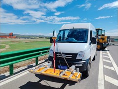
a) 3D GPR Inspection vehicle

b) Harbor inspection location

c) Data processing

3. Experimental results and analysis

The forward simulation data is processed using MATLAB to perform three-dimensional reconstruction, followed by in-depth analysis from three dimensions: B-scan direction slicing analysis, Sobel edge detection feature extraction from the top-down view, and spectrum analysis perpendicular to the B-scan direction. Then, for the artificially embedded field defects, the analysis is carried out based on reflection wave characteristics, co-phase axes, and waveform features. Finally, a comparative analysis is conducted between the simulated data and field measurement data to derive the radar spectral features of interlayer bonding defects.

3.1. 3D forward simulation results

3.1.1. Forward simulation of base and subbase bonding zones

3.1.1.1. B-scan direction slicing of forward simulation at different moisture contents for defect sizes 10×20×3 and 20×20×3

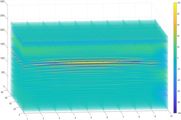
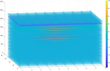
For the forward simulation results of the bonding zone between the base and subbase, the B-scan direction radar response characteristics were studied for defect sizes of 10×20×3 and 20×20×3 under different moisture contents. As the defect size increases, the radar signal reflection becomes stronger. As shown in Fig. 5, the co-phase axis of the reflected signal is discontinuous. Under low moisture conditions, the radar wave reflection is relatively weak, but the radar reflection in the defect area is more prominent, allowing the distinction of the defect size and layer position. In Fig. 6, the reflected signal is enhanced compared to Fig. 5, with the reflection anomaly in the defect area becoming more evident. The defect area appears as a clearer high-reflection region, with the boundary becoming more defined. The increased moisture content makes the electromagnetic properties of the defect area more distinct, improving the detection accuracy of the defect. As seen in Fig. 7, the reflected signal is further strengthened, with the defect area showing a very obvious high-reflection region. The boundary of the defect area is clearer, and the intensity of the reflection signal is noticeably higher than in the surrounding normal areas. The increase in moisture content continues to enhance defect detection, but may also complicate the reflection signal. Fig. 8 shows the strongest reflected signal, with the defect area exhibiting a very high reflection intensity. The contrast between the defect area and the surrounding normal areas is very obvious, with the boundary extremely clear.

Fig. 5Forward simulation B-scan slice in the direction of 5 % moisture content

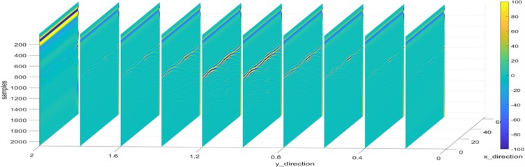
Fig. 6Forward simulation B-scan slice in the direction of 10 % moisture content

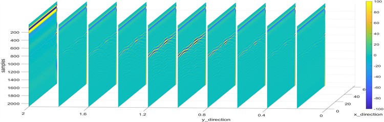
Fig. 7Forward simulation B-scan slice in the direction of 15 % moisture content

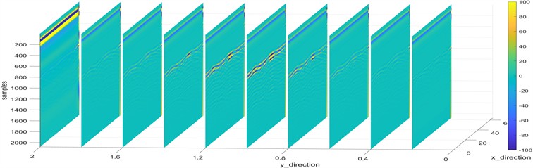
Fig. 8Forward simulation B-scan slice in the direction of 25 % moisture content

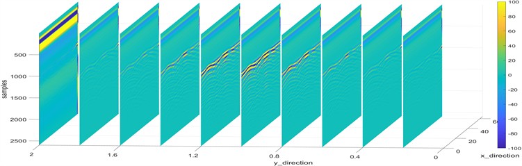
By analyzing the forward simulation results at different moisture contents, the following conclusions can be drawn:

In the B-scan direction, increasing the moisture content enhances the radar wave’s reflection signal, thereby improving the detection effect of the defect area.

At higher moisture contents (e.g., 25 %), the radar reflection characteristics of the defect area are most prominent, and the boundary is clear, making it easier to identify. However, this may also lead to signal complexity, requiring more sophisticated signal processing methods.

An optimal moisture content (e.g., 10 %-15 %) provides a balanced detection effect, enabling clear identification of the defect area while avoiding overly complex reflection signals.

3.1.1.2. 3D reconstruction top-down view for defect sizes 10×20×3 and 20×20×3 at different moisture contents

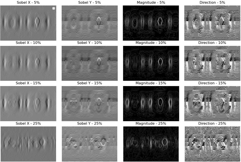
The Sobel edge detection algorithm was used for feature extraction for Figs. 9-12, which specifically includes calculating the gradient in the Sobel $X$ -direction and $Y$ -direction, the gradient magnitude, and the direction of the gradient to be able to visualize the radar mapping features.

Fig. 93D reconstruction top view of 5 % moisture content

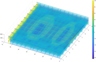
Fig. 103D reconstruction top view of 10 % moisture content

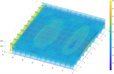
Fig. 113D reconstruction top view of 15 % moisture content

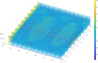
Fig. 123D reconstruction top view of 25 % moisture content

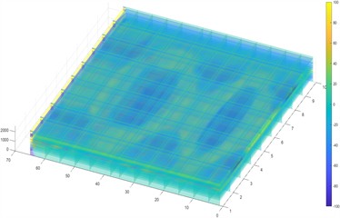
Fig. 13 shows that, for both damage sizes, Sobel X and Sobel Y demonstrate the gradients of the image in the horizontal and vertical directions. As the moisture content increases, the gradient intensities of Sobel X and Y become more pronounced. However, at a high moisture content of 25 %, the scattering effect is enhanced, leading to signal clutter, which makes the edge information less clear.

Fig. 13Feature extraction image using Sobel edge detection algorithm

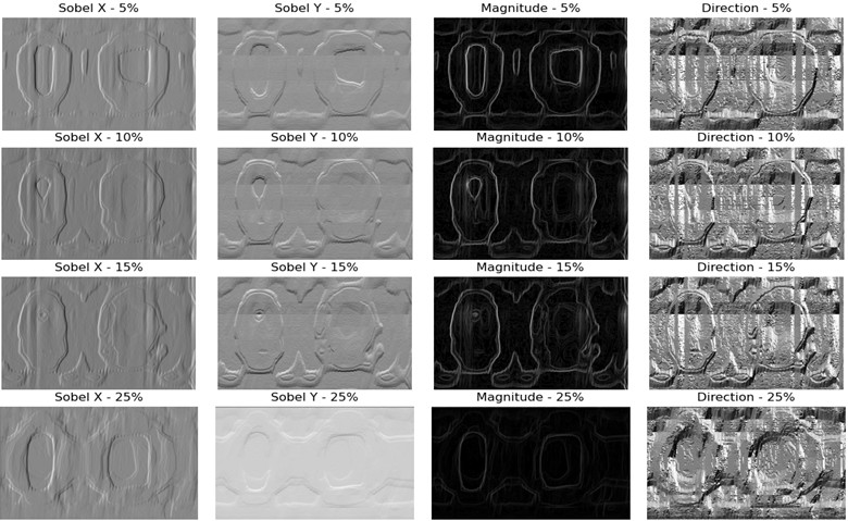
The Magnitude represents the gradient magnitude, which reflects the combined impact of Sobel X and Y gradients. As the moisture content increases from 5 % to 15 %, the gradient magnitude map shows more distinct and clearer edge lines, while the central area gradually decreases, presenting a “layered” pattern. This indicates that increased moisture content enhances the contrast between material interfaces and internal structures in the radar image, making the edges more prominent. However, at 25 % moisture content, increased water may lead to an enhancement of scattering effects, especially when the moisture distribution is uneven. This added scattering can interfere with the normal propagation and reflection of radar waves, and with the processing of radar images, the complexity of the high moisture signal increases, causing blurring of image details and loss of edge information.

Gradient direction (Direction) represents the direction of the edges, shown by different grayscale values. The increase in moisture content leads to more complex textures and pattern variations in the gradient direction map, which may be caused by the presence of moisture affecting the radar wave propagation path, thereby altering the direction of the reflected waves.

By comparing the images at different moisture contents, it can be observed that as the moisture content increases, the edge intensity and clarity of the image increase. This is due to changes in material density and dielectric constant caused by the increased moisture content, which enhances the reflection and scattering of radar waves. Higher moisture content makes the image textures and internal structures more complex and evident. The increased complexity in the gradient direction may reflect the uneven distribution of moisture or the complex response of the internal structure of the material, leading to the blurring of image details and the loss of edge information.

3.1.1.3. Three-dimensional reconstruction of B-scan direction images at different moisture contents for damage sizes of 10×20×3 and 20×20×3

Figs. 14 to 17 show that after three-dimensional reconstruction in the vertical B-scan direction, a “banded” pattern is presented. As the moisture content increases, the radar reflection signal gradually intensifies, following a similar trend to Figs. 5 to 8. The delaminated or poorly bonded areas are characterized by discontinuous or broken reflection lines. This occurs because the reflection properties of radar waves change when they encounter interfaces between different materials. Additionally, as the moisture content increases, the reflection intensity in well-bonded areas is typically more uniform, while in poorly bonded areas, the reflection intensity may significantly increase due to inconsistent material density and moisture, reflecting enhanced radar wave reflection and scattering. A moderate moisture content improves the image contrast and detail, while excessive moisture content leads to a degradation in image quality due to scattering and absorption effects.

Fig. 145 % moisture content 3D reconstruction vertical B-scan directional image

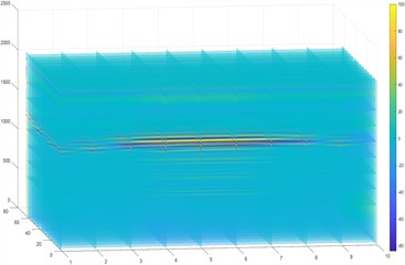
Fig. 1510 % moisture content 3D reconstruction vertical B-scan directional image

Fig. 1615 % moisture content 3D reconstruction vertical B-scan directional image

Fig. 1725 % moisture content 3D reconstruction vertical B-scan directional image

3.1.2. Pavement surface and base layer bonding simulation

3.1.2.1. B-scan direction slices of forward simulation with damage sizes of 10×20×3 and 20×20×3 under different moisture contents

Figs. 18 to 21 show the forward simulation results for the pavement surface and base layer bonding, where the radar response characteristics in the B-scan direction were studied for damage sizes of 10×20×3 and 20×20×3 under different moisture contents. Poorly bonded areas typically exhibit fractured or discontinuous reflection lines. This phenomenon occurs because radar waves encounter different obstacles and reflections when passing through uneven interfaces. Due to the physical property differences in the materials of the poorly bonded regions, the radar wave propagation speed becomes uneven. In the B-scan images, this is represented as waveform curvature or irregular spreading, leading to multiple reflections of the radar wave and forming a multi-layer echo phenomenon. In radar images, this appears as repeated reflection signals, which may sometimes obscure or confuse the actual interface signals. As the moisture content increases from 5 % to 25 %, the radar signals gradually intensify.

Fig. 185 % moisture content forward simulation B-scan directional slice image

Fig. 1910 % moisture content forward simulation B-scan directional slice image

Fig. 2015 % moisture content forward simulation B-scan directional slice image

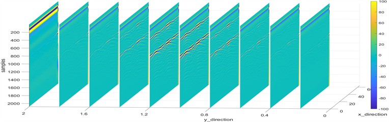
Fig. 2125 % moisture content forward simulation b-scan directional slice image

Through analysis of the forward simulation results under different moisture contents, it can be concluded that:

An increase in moisture content enhances the reflection signal of radar waves, improving the detection of damage areas. At 25 % moisture content, the radar reflection characteristics of the damage area are most pronounced, with clear boundaries that make it easier to identify. However, this can also lead to signal complexity, requiring more advanced signal processing methods to avoid misjudgment and improve damage recognition. Moisture content levels of 10 %-15 % provide a more balanced detection effect, clearly identifying damage areas while avoiding interference from overly complex reflection signals.

3.1.2.2. Three-dimensional reconstructed top-down view of the forward simulation with damage sizes of 10×20×3 and 20×20×3 under different moisture contents

To more intuitively highlight the radar signature features, the Sobel edge detection algorithm was applied to Figs. 22, 23, 24, and 25 for feature extraction. This process includes calculating the Sobel gradients in the $X$ and $Y$ directions, gradient magnitude, and gradient direction, in order to visually display the radar signature characteristics.

Fig. 223D reconstruction top view of 5% moisture content

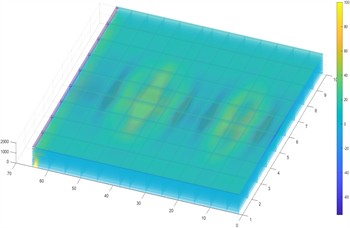
Fig. 233D reconstruction top view of 10 % moisture content

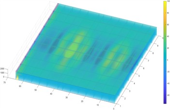
Fig. 243D reconstruction top view of 15 % moisture content

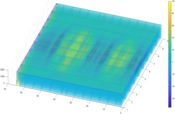
Fig. 253D reconstruction top view of 25 % moisture content

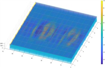
Fig. 26Sobel edge detection algorithm feature extraction map

As shown in Fig. 26, Sobel X and Y direction gradients: The Sobel X direction gradient emphasizes edges in the image that are perpendicular to the $X$ -axis, while the $Y$ direction gradient highlights edges perpendicular to the $Y$ -axis. As the moisture content increases, the gradient intensities in both directions increase, revealing more details and interfaces. When the moisture content is between 5 % and 15 %, the gradients are clearly visible, and the edge lines are sharp. However, when the moisture content increases to 25 %, the scattering effect intensifies, leading to signal clutter and blurry edge information, indicating the loss of gradient information at higher moisture levels.

Gradient magnitude and direction: From low to medium moisture content, the gradient magnitude shows clear edges and “layered” patterns, indicating enhanced contrast between material interfaces and internal structures. However, at 25 % moisture content, the gradient magnitude becomes blurred due to increased moisture scattering. The gradient direction map shows more complex textures and pattern changes as the moisture content increases, which may be due to moisture affecting the radar wave propagation path and altering the direction of the reflected waves.

Through comparative analysis of the images at different moisture contents, it can be concluded that an increase in moisture content typically enhances the variations in material density and dielectric constant, thereby strengthening the reflection and scattering of radar waves. However, the scattering effect at high moisture content may cause a loss of image details and blurred edge information, which requires more detailed parameter adjustments and analysis in practical applications to ensure data accuracy and reliability.

3.1.2.3. Three-dimensional reconstruction of the vertical B-scan direction for defect sizes 10×20×3 and 20×20×3 at different moisture contents

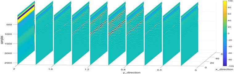
From Figs. 27 to 30, it can be observed that the vertical B-scan direction, after three-dimensional reconstruction, presents a “banded” pattern. Under normal conditions, areas with good bonding between the surface and the base layer display continuous and smooth reflection waveforms. In areas with poor bonding, the discontinuity of the reflection waveform becomes apparent, showing clear breaks or interruptions. As the moisture content increases, the reflection intensity in the well-bonded areas is generally more uniform. However, in the poorly bonded regions, due to inconsistencies in material density, humidity, and the inhomogeneity of materials at the interfaces, the waveform may become distorted or deformed, and the reflection intensity may significantly increase, indicating enhanced radar wave reflection and scattering.

Fig. 275 % moisture content 3D reconstruction vertical B-scan directional image

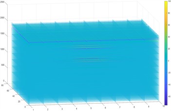
Fig. 2810 % moisture content 3D reconstruction vertical B-scan directional image

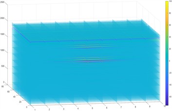
Fig. 2915 % moisture content 3D reconstruction vertical B-scan directional image

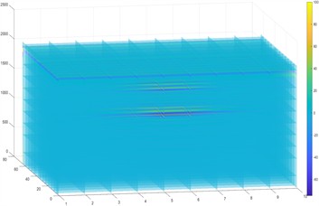
Fig. 3025 % moisture content 3D reconstruction vertical B-scan directional image

3.2. Embedded defect data collection

In this experiment, defects were embedded in the emergency parking zone of a harbor, and three-dimensional ground-penetrating radar (GPR) was used for detection. The equipment parameters were set as follows: a sampling interval of 4.96 cm, dwell time of 2 ns, and speed of 10 km/h. Images with good quality were selected. The following radar characteristic images represent interlayer bonding defects with varying layer positions, defect sizes, and moisture contents. The analysis focuses on the reflection wave characteristics, phase axis, and waveform of the defects.

3.2.1. Measured results of the bonding between the base and subbase layers

Measured results for defect size 10×20×3 at different moisture contents shown in Table 5.

Measured results for defect size 20×20×3 at different moisture contents shown in Table 6.

From Tables 5 and 6, it can be seen that by comparing the three-dimensional radar images at different moisture contents for two defect sizes, the B-scan images are used to display the distribution of reflection intensity along the radar scan line, reflecting the characteristics of radar wave reflection as it passes through the defect areas. The A-scan images provide the reflection waveform at specific locations, typically used to analyze the waveform characteristics. As the moisture content increases, the phase axis of the defect area in the B-scan image breaks and curves, and the reflection intensity gradually increases, altering the shape and intensity of the reflection waveform.

Table 5Measured results for different moisture contents with disease size 10×20×3

Group 1	Image A	Image B	Image C	Image D
Moisture content	5 %	10 %	15 %	Post-water addition 25 %
Measured B-scan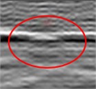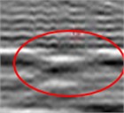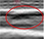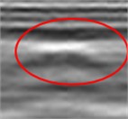
A-scan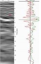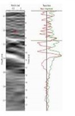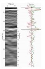
Horizontal plane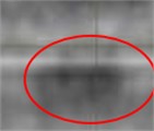

Table 6Measured results for different moisture contents with disease size 20×20×3

Group 2	Image A	Image B	Image C	Image D
Moisture content	5 %	10 %	15 %	Post-water addition 25 %
Measured B-scan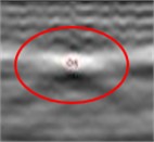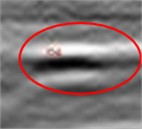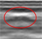
A-scan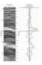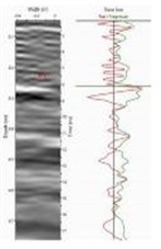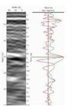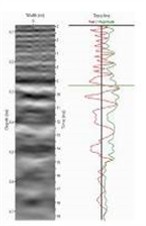
Horizontal plane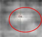

This effect is especially evident in the defect area, where the reflection wave peak and amplitude become more pronounced. In the radar images, this phenomenon is particularly noticeable and can help pinpoint the problem areas. From the A-scan waveforms, it can be seen that in the poorly bonded regions, the reflection waveform also changes, showing waveform distortion and sudden amplitude variations. This phenomenon is particularly clear in the A-scan images and serves as an important feature for identifying poor bonding. From the top-down view, it is observed that as the moisture content increases from 5 % to 15 %, the reflection areas for both defect sizes become more pronounced. However, in the later stage with higher moisture content (25 %), when combined with the A-scan waveform, the reflections weaken to some extent. This is due to the enhanced scattering effects, leading to chaotic signals and blurred edge information, indicating that higher moisture content causes some loss of radar data. By analyzing the three-dimensional radar data, defect size, moisture content, and interlayer bonding conditions have a significant impact on the radar images.

3.2.2. Measured results of the bonding between the surface and the base layer

Measured results for defect size 10×20×3 at different moisture contents shown in Table 7.

Measured results for defect size 20×20×3 at different moisture contents shown in Table 8.

Table 7Measured results for different moisture contents with disease size 10×20×3

Group 3	Image A	Image B	Image C	Image D
Moisture content	5 %	10 %	1 5%	Post-water addition 25 %
Measured B-scan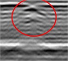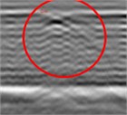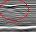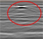
A-scan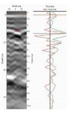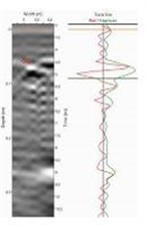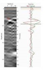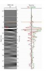
Horizontal plane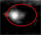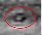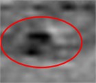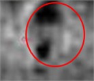

From Tables 7 and 8, it can be seen that interlayer bonding defects exhibit different reflection intensities at different moisture contents. At a moisture content of 5 %, the defect is similar to the asphalt pavement base layer, but contains some air inside. When electromagnetic waves propagate through sandy soil, the defect appears as a distorted pattern with alternating light and dark areas on the radar image due to the difference in dielectric constants. At a moisture content of 10 %, the defect’s moisture content is higher than that of the base layer. Because the dielectric constant of water is stable and distributed uniformly within the defect, a strong reflective hyperbolic pattern appears at the top of the defect in the electromagnetic wave’s longitudinal section, covering part of the lower radar image. In the horizontal cross-section, the defect location shows a strong reflection.

From the waveform at the defect location, it can be observed that the amplitude of the defect waveform is larger due to the difference in dielectric constants. As the moisture content increases, especially after exceeding 10 %, the amplitude and period of the defect waveform increase significantly. This is closely related to the increased electrical conductivity due to the higher water content inside the defect. Overall, there is a certain linear relationship between the amplitude and period of the waveform and the water content.

Table 8Measured results for different moisture contents with disease size 20×20×3

Group 4	Image A	Image B	Image C	Image D
Moisture content	5 %	10 %	15 %	Post-water addition 25 %
Measured B-scan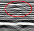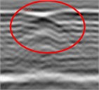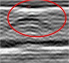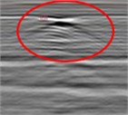
A-scan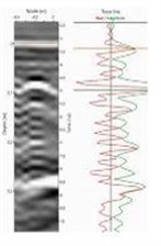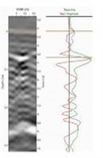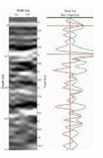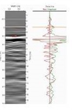
Horizontal plane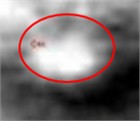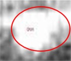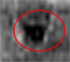

The clarity of the interlayer bonding defect image, as well as the amplitude and frequency of the waveform, is significantly affected by the depth. Comparing the interlayer bonding defects at the base and subbase layers, it can be found that defects located at the base-subbase interface, due to their deeper depth, experience a greater impact on signal strength after the radar’s electromagnetic waves are reflected by the defect. This is especially true for defects with a moisture content exceeding 15 %, where the amplitude and frequency of the waveform show noticeable attenuation. This indicates that the diffraction signals of the defect waveform at the base-subbase interface are significantly weakened, and the increased moisture content enhances the scattering effects, particularly when the moisture distribution is uneven. The increased scattering may interfere with the normal propagation and reflection of radar waves.

Since the electromagnetic waves emitted by the radar have shorter wavelengths, they have weaker penetration capabilities but higher resolution. When defects are located deeper, the energy of short-wavelength electromagnetic waves is significantly attenuated after passing through the asphalt pavement base layer and reflecting multiple times within the defect. As a result, the quality of the high-frequency electromagnetic waves received by the radar is poor. Although low-frequency electromagnetic waves experience less energy loss, their accuracy is lower, leading to slight discrepancies in the detection of defect sizes at greater depths.

3.3. Comprehensive comparative analysis

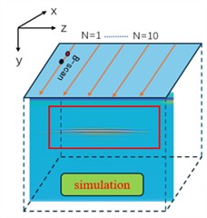
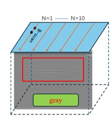
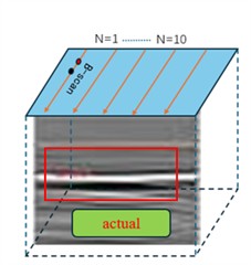
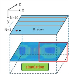
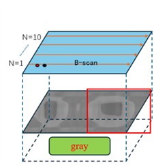
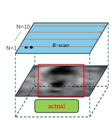
Based on Figs. 31-33, it can be observed that the actual measured data and simulated data exhibit good overall similarity in interlayer bonding defects, with consistent radar pattern features.

The B-scan directional image displays the radar reflection waveform along a specific cross-sectional direction. By comparison, it can be observed that the simulated and measured images show relatively consistent reflection intensity and waveform characteristics in most areas. Images perpendicular to the B-scan direction present the propagation and reflection characteristics of radar waves in another cross-sectional direction. The simulated and measured images also exhibit high similarity in major structural features. The top-view image provides a planar radar reflection waveform view, showing the overall characteristics of the entire detection area. From the top-view perspective, the simulated and measured results show a high degree of agreement in large-scale features, such as the main distribution of reflection intensity and overall waveform shape.

Fig. 31Comparison between simulated and measured B-scan direction

a) Simulation chart

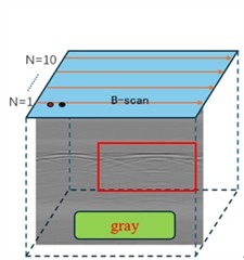
b) Grayscale chart

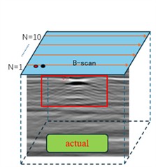
c)Actual chart

Fig. 32Comparison between simulated and measured vertical B-scan direction

a) Simulation chart

b) Grayscale chart

c)Actual chart

Fig. 33Comparison between simulated and measured top-down view

a) Simulation chart

b) Grayscale chart

c) Actual chart

Across three dimensions, the simulated images have a cleaner background, while the measured images contain clutter and noise. Although the measured data were processed using post-processing software after data acquisition, the processed results still show discrepancies compared to the simulated images. The primary reason for this difference lies in the fact that the simulated model was designed using the #soil_peplinski and #fractal_box material commands of the gprMax software. These commands effectively reflect the macroscopic properties of the materials, but due to the idealized assumptions of the model, they fail to simulate the microscopic heterogeneities within the materials (e.g., cracks, air bubbles, particle distribution) and irregular interfacial bonding properties. These microscopic factors can lead to localized dielectric constant fluctuations, enhanced scattering, and multiple reflections, thereby generating subtle clutter in the measured data. Furthermore, the complexity of material uniformity and interfacial bonding conditions during actual construction, as well as equipment noise and external environmental interference, further exacerbate the generation of background noise.

Based on the discussion above, Table 9 summarizes the radar characteristic maps of typical hidden defects in asphalt pavement and the influence of various factors.

Table 9Radar characteristic spectrum of typical hidden defects in asphalt pavement and the influence of different factors

Defect type	Defect description	Influence of depth	Influence of moisture content	Influence of size
Normal asphalt pavement	Clear structural layering, continuous phase axis with no breaks and strong reflections	–	–	–
Poor interlayer bonding	Discontinuous phase axis. A “banded” pattern appears in the vertical B-scan direction; a “downward bending” reflection pattern in B-scan; a “patchy area” pattern in the top view	The deeper the defect, the more blurred the radar characteristic spectrum, and the lower the amplitude of the waveform	As the moisture content increases, the reflection intensity at the defect site increases. A moderate moisture content provides a more balanced detection result	The larger the defect size, the larger the area of the defect in the radar characteristic spectrum, and the right-angled defect contour becomes more rounded

4. Engineering validation of interlayer bonding defects

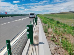
Based on the previous research findings, the detection was conducted on the section of the An-Gong Expressway, Segment 1. This section starts at the eastern end of Anye Village and ends near Gongzhugeng, passing through Zhengxiangbaiqi and Zhengxianglanqi. The total length of the route is 178 km, with a designed speed of 120 km/h, a roadbed width of 25.5 m, and a dual four-lane layout. Construction began in 2002, and the entire line was completed and opened to traffic in 2005. As of now, the road has been in operation for over 15 years, with some sections experiencing serious damage to the asphalt pavement surface and base layers.

Three-dimensional Ground Penetrating Radar (GPR) was used for detection. The equipment parameters were set as follows: sampling interval of 4.96 cm, dwell time of 2 ns, speed of 10 km/h, and the positioning system used was the RTK produced by Zhonghaida Company. The detected section of the road is between mile markers K190+000 and K209+400, with a minimum detection unit length of 100 meters, totaling 19.4 km. An 11 km section was selected for detailed analysis of the asphalt pavement base and sub-base layers. The types of defects detected were interlayer bonding defects, which were measured, identified, and statistically analyzed. The detection images are shown in Table 10.

Based on the previous research findings, core sampling was conducted at the locations corresponding to the radar feature maps, as shown in Fig. 34. The results confirmed the existence of interlayer bonding defects of varying degrees, as indicated in Figs. 2-4. This validated the effectiveness of radar technology in identifying and assessing internal defects and diseases within roads, thus providing a reliable scientific basis for the application of radar technology in road inspection. This study makes an important contribution to the early detection and resolution of interlayer bonding issues, thereby extending the service life of roads.

Table 10Radar mapping of actual detected road sections

Pile number	Defect length	Defect type	Radar characteristic spectrum
K193+700	36 m	Poor interlayer bonding in subbase and base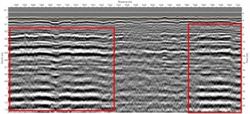
K198+200	37 m	Poor interlayer bonding in subbase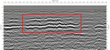
K198+400	20 m	Poor interlayer bonding in subbase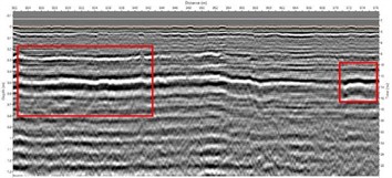
K199+300	30m	Poor interlayer bonding in subbase and base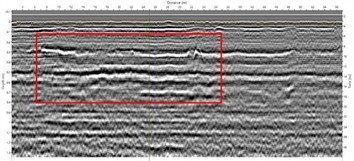
K203+700	45m	Poor interlayer bonding in subbase and base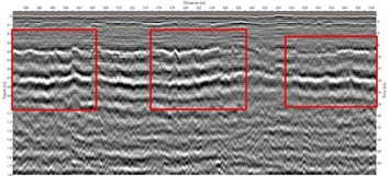
K205+400	49m	Poor interlayer bonding between base and subbase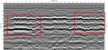
K208+600	22m	Poor interlayer bonding in subbase and slight bonding issues in base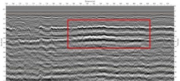

Fig. 34Sampling of poor interlayer bonding

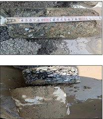
a) Disease chart

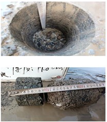
b) Disease chart

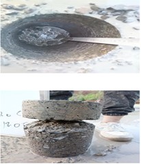
c) Disease char t

5. Conclusions

This study employed gprMax forward numerical simulations, artificial defect placement methods, and engineering verification to investigate the radar features of interlayer bonding defects at different moisture contents and defect sizes for both surface-base and base-subbase layers. The main conclusions are as follows:

1) Increased Moisture Content Enhances Reflective Signals: When the moisture content is between 5 % and 15 %, it provides a balanced detection effect, allowing clear identification of defect areas while avoiding excessive interference from complex reflective signals. However, moisture content exceeding 25 % can lead to signal complexity, requiring more advanced signal processing methods to avoid misinterpretation, which may affect defect identification.

2) Radar Characteristics of Interlayer Bonding Defects: Interlayer bonding defects in radar images are characterized by discontinuities in the same-phase axis. In the B-scan direction, the reflection pattern presents a slight “downward curve”, while in the vertical B-scan direction, a “banded” pattern appears. In the horizontal top-down view, the defect shows a “sheet-like area” pattern.

3) Depth-dependent radar features: The radar feature map becomes more blurred with increased defect depth. The waveform amplitude decreases with depth, and the defect area increases with size. As the defect shape becomes more pronounced, the corners of the rectangular defect contours tend to round.

4) Through comparative analysis of the simulated and measured data across three dimensions, it was found that the simulated results are consistent with the measured data in overall characteristics (reflection intensity distribution and waveform shape). However, at radar defect features, there is subtle background clutter and noise, mainly caused by the idealization of the model and the complexity of actual pavement structures. It is recommended to improve and develop more comprehensive and advanced models in the future, and to enhance the overall evaluation capability of radar detection through multidimensional data fusion.

References

W. Yuya, T. Yasushi, K. Futoshi, and W. Kazuhiro, “Evaluation of the effect of interlayer bonding condition on the deterioration of asphalt pavement,” Transportation Research Record: Journal of the Transportation Research Board, Vol. 2677, No. 7, pp. 500–508, Feb. 2023, https://doi.org/10.1177/03611981231153649

Publisher
J. Zhu, M. Lei, and Y. Liu, “Study on pull-out test between base and surface layers of asphalt pavement,” Transportation Science and Technology, No. 1, pp. 75–78, 2013.

Search CrossRef
Y. Wang and Y. Yang, “A review of interlayer bonding detection technology for asphalt pavement,” Highway Transportation Science and Technology (Applied Technology Edition), Vol. 5, No. 7, pp. 21–23, 2009.

Search CrossRef
A. B. Crusho and S. Niveditha, “A state-of-art review on the interfacial bond strength of bituminous overlay in asphalt pavements,” International Advance Journal of Engineering Research, Vol. 3, No. 3, pp. 20–26, 2020.

Search CrossRef
A. Vaitkus, D. Žilionienė, S. Paulauskaitė, F. Tuminienė, and L. Žiliūtė, “Research and assessment of asphalt layers bonding,” The Baltic Journal of Road and Bridge Engineering, Vol. 6, No. 3, pp. 210–218, Sep. 2011, https://doi.org/10.3846/bjrbe.2011.27

Publisher
H. Wang, G. Xu, Z. Wang, and T. Bennert, “Flexible pavement interface bonding: theoretical analysis and shear-strength measurement,” Journal of Testing and Evaluation, Vol. 46, No. 1, pp. 99–107, Jan. 2018, https://doi.org/10.1520/jte20160288

Publisher
F. Canestrari et al., “Mechanical testing of interlayer bonding in asphalt pavements,” in Advances in Interlaboratory Testing and Evaluation of Bituminous Materials, RILEM State-of-the-Art Reports, Dordrecht: Springer Netherlands, 2012, pp. 303–360, https://doi.org/10.1007/978-94-007-5104-0_6

Publisher
K. Yang and R. Li, “Characterization of bonding property in asphalt pavement interlayer: A review,” Journal of Traffic and Transportation Engineering (English Edition), Vol. 8, No. 3, pp. 374–387, Jun. 2021, https://doi.org/10.1016/j.jtte.2020.10.005

Publisher
J. P. Giri and M. Panda, “Laboratory evaluation of inter-layer bond strength between bituminous paving layers,” Transportation Infrastructure Geotechnology, Vol. 5, No. 4, pp. 349–365, Sep. 2018, https://doi.org/10.1007/s40515-018-0064-z

Publisher
D. Shang, “Study on the evaluation of interlayer bonding effect in asphalt pavement surface,” (in Chinese), Northeast Forestry University, 2011.

Search CrossRef
H. M. Akraym, R. Muniandy, F. M. Jakarni, and S. Hassim, “Review: shear properties and various mechanical tests in the interface zone of asphalt layers,” Infrastructures, Vol. 8, No. 3, p. 48, Mar. 2023, https://doi.org/10.3390/infrastructures8030048

Publisher
L. Zou, L. Yi, and M. Sato, “On the use of lateral wave for the interlayer debonding detecting in an asphalt airport pavement using a multistatic GPR system,” IEEE Transactions on Geoscience and Remote Sensing, Vol. 58, No. 6, pp. 4215–4224, Jun. 2020, https://doi.org/10.1109/tgrs.2019.2961772

Publisher
P. Shangguan and I. L. Al-Qadi, “Calibration of FDTD simulation of GPR signal for asphalt pavement compaction monitoring,” IEEE Transactions on Geoscience and Remote Sensing, Vol. 53, No. 3, pp. 1538–1548, Mar. 2015, https://doi.org/10.1109/tgrs.2014.2344858

Publisher
X. Dérobert, V. Baltazart, J.-M. Simonin, S. S. Todkar, C. Norgeot, and H.-Y. Hui, “GPR monitoring of artificial debonded pavement structures throughout its life cycle during accelerated pavement testing,” Remote Sensing, Vol. 13, No. 8, p. 1474, Apr. 2021, https://doi.org/10.3390/rs13081474

Publisher
J. Yang, S. Yang, Y. Yao, J. Gao, and S. Wang, “Three-dimensional orthorectified simulation and ground penetrating radar detection of interlayer bonding condition in asphalt pavements,” Measurement Science and Technology, Vol. 35, No. 9, p. 095017, Sep. 2024, https://doi.org/10.1088/1361-6501/ad57d8

Publisher
C. Guo, F. Wang, and Y. Zhong, “Assessing pavement interfacial bonding condition,” Construction and Building Materials, Vol. 124, pp. 85–94, Oct. 2016, https://doi.org/10.1016/j.conbuildmat.2016.07.064

Publisher
A. Rahman, C. Ai, C. Xin, X. Gao, and Y. Lu, “State-of-the-art review of interface bond testing devices for pavement layers: toward the standardization procedure,” Journal of Adhesion Science and Technology, Vol. 31, No. 2, pp. 109–126, Jan. 2017, https://doi.org/10.1080/01694243.2016.1205240

Publisher
S. Wang, J. Ning, and Z. Wang, “FDTD-based forward analysis for detection of protective layer on coal seam working face,” Mining Technology, Vol. 20, No. 1, pp. 145–149, 2020, https://doi.org/10.3969/j.issn.1671-2900.2020.01.042

Publisher
J. Li, H. Lu, and M. Li, “Effects of temperature and moisture on the bonding performance of porous asphalt pavement interlayers,” Highway Engineering, Vol. 46, No. 5, pp. 144–148, 2021, https://doi.org/10.19782/j.cnki.1674-0610.2021.05.022

Publisher
P. Chaturabong and H. U. Bahia, “Effect of moisture on the cohesion of asphalt mastics and bonding with surface of aggregates,” Road Materials and Pavement Design, Vol. 19, No. 3, pp. 741–753, Apr. 2018, https://doi.org/10.1080/14680629.2016.1267659

Publisher
A. C. Raposeiras, D. Castro-Fresno, A. Vega-Zamanillo, and J. Rodriguez-Hernandez, “Test methods and influential factors for analysis of bonding between bituminous pavement layers,” Construction and Building Materials, Vol. 43, pp. 372–381, Jun. 2013, https://doi.org/10.1016/j.conbuildmat.2013.02.011

Publisher
H. Hou and B. Qin, “Forward simulation of road void detection using GprMax,” Transportation Energy and Environmental Protection, Vol. 20, No. 2, pp. 157–161, 2024, https://doi.org/10.3969/j.issn.1673-6478.2024.02.031

Publisher
Y. X. Li, X. T. Kang, S. M. Sheng, and C. J. Fu, “Characterization of 3D-radar images of pavement devoid damage based on FDTD,” Journal of Measurements in Engineering, Vol. 11, No. 4, pp. 467–481, Dec. 2023, https://doi.org/10.21595/jme.2023.23469

Publisher
Q. Ye, “GPR-based structure feature extraction and defect identification of roadbed,” (in Chinese), Nanjing University of Posts and Telecommunications, 2019.

Search CrossRef
L. Wang, X. Gu, Z. Liu, W. Wu, and D. Wang, “Automatic detection of asphalt pavement thickness: A method combining GPR images and improved Canny algorithm,” Measurement, Vol. 196, p. 111248, Jun. 2022, https://doi.org/10.1016/j.measurement.2022.111248

Publisher
Y. Pan, X. Chen, Q. Sun, and X. Zhang, “Monitoring asphalt pavement aging and damage conditions from low-altitude UAV imagery based on a CNN approach,” Canadian Journal of Remote Sensing, Vol. 47, No. 3, pp. 432–449, May 2021, https://doi.org/10.1080/07038992.2020.1870217

Publisher
A. de Coster et al., “Towards an improvement of GPR-based detection of pipes and leaks in water distribution networks,” Journal of Applied Geophysics, Vol. 162, pp. 138–151, Mar. 2019, https://doi.org/10.1016/j.jappgeo.2019.02.001

Publisher
N. Kheradmandi and V. Mehranfar, “A critical review and comparative study on image segmentation-based techniques for pavement crack detection,” Construction and Building Materials, Vol. 321, p. 126162, Feb. 2022, https://doi.org/10.1016/j.conbuildmat.2021.126162

Publisher

About this article

Received

20 August 2024

Accepted

26 January 2025

Published

27 February 2025

DOI

https://doi.org/10.21595/jme.2025.24466

Keywords

poor interlayer bonding

3D radar

forward simulation

characterization

Acknowledgements

This research was sponsored by the Construction Science and Technology Project (NJ-2021-15) of the Department of Transportation of Inner Mongolia Autonomous Region.

Data Availability

The datasets generated during and/or analyzed during the current study are available from the corresponding author on reasonable request.

Author Contributions

Yongxiang Li: conceptualization, formal analysis, funding acquisition, supervision, validation, writing-review and editing; Fa Chen: investigation, methodology, software, visualization, writing-original draft preparation; Changjiang Fu: project administration; Shaomeng Sheng and Xiatong Kang: resources.

Conflict of interest

The authors declare that they have no conflict of interest.

This is an open access article distributed under the Creative Commons Attribution License, which permits unrestricted use, distribution, and reproduction in any medium, provided the original work is properly cited.

Y. X. Li, F. Chen, C. J. Fu, S. M. Sheng, and X. T. Kang, “3D GPR profile analysis of interlayer bonding failure in asphalt pavement based on FDTD,” Journal of Measurements in Engineering, Vol. 13, No. 2, –24, Feb. 2025, https://doi.org/10.21595/jme.2025.24466

Copy Extrica

Copied to clipboard!

TY  - JOUR
DO  - 10.21595/jme.2025.24466
UR  - https://doi.org/10.21595/jme.2025.24466
TI  - 3D GPR profile analysis of interlayer bonding failure in asphalt pavement based on FDTD
T2  - Journal of Measurements in Engineering
AU  - Li, Y. X.
AU  - Chen, F.
AU  - Fu, C. J.
AU  - Sheng, S. M.
AU  - Kang, X. T.
PY  - 2025
DA  - 2025/02/27
PB  - Extrica
VL  - 13
IS  - 2
SN  - 2335-2124
SN  - 2424-4635
ER  - 

Copy Ris

Copied to clipboard!

 @article{Li_2025, title={3D GPR profile analysis of interlayer bonding failure in asphalt pavement based on FDTD}, ISSN={2424-4635}, url={https://doi.org/10.21595/jme.2025.24466}, DOI={10.21595/jme.2025.24466}, journal={Journal of Measurements in Engineering}, publisher={JVE International Ltd.}, author={Li, Y. X. and Chen, F. and Fu, C. J. and Sheng, S. M. and Kang, X. T.}, year={2025}, month=feb }

Copy Bibtex

Copied to clipboard!

[1]Y. X. Li, F. Chen, C. J. Fu, S. M. Sheng, and X. T. Kang, “3D GPR profile analysis of interlayer bonding failure in asphalt pavement based on FDTD,” Journal of Measurements in Engineering, Feb. 2025, doi: 10.21595/jme.2025.24466.

Copy IEEE

Copied to clipboard!

Li, Y. X., F. Chen, C. J. Fu, S. M. Sheng, and X. T. Kang. “3D GPR Profile Analysis of Interlayer Bonding Failure in Asphalt Pavement Based on FDTD.” Journal of Measurements in Engineering, February 27, 2025. https://doi.org/10.21595/jme.2025.24466.

Copy Chicago

Copied to clipboard!

3D GPR profile analysis of interlayer bonding failure in asphalt pavement based on FDTD

Abstract

1. Introduction

2. Experimental methods

2.1. FDTD forward simulation methodology

2.1.1. Forward simulation process

2.1.2. Forward model design

2.2. Artificial disease field deployment methods

2.3. Three-dimensional radar data acquisition and processing

2.3.1. Sobel algorithm for edge detection

2.3.2. Gradient magnitude and direction calculation

3. Experimental results and analysis

3.1. 3D forward simulation results

3.1.1. Forward simulation of base and subbase bonding zones

3.1.1.1. B-scan direction slicing of forward simulation at different moisture contents for defect sizes 10×20×3 and 20×20×3

3.1.1.2. 3D reconstruction top-down view for defect sizes 10×20×3 and 20×20×3 at different moisture contents

3.1.1.3. Three-dimensional reconstruction of B-scan direction images at different moisture contents for damage sizes of 10×20×3 and 20×20×3

3.1.2. Pavement surface and base layer bonding simulation

3.1.2.1. B-scan direction slices of forward simulation with damage sizes of 10×20×3 and 20×20×3 under different moisture contents

3.1.2.2. Three-dimensional reconstructed top-down view of the forward simulation with damage sizes of 10×20×3 and 20×20×3 under different moisture contents

3.1.2.3. Three-dimensional reconstruction of the vertical B-scan direction for defect sizes 10×20×3 and 20×20×3 at different moisture contents

3.2. Embedded defect data collection

3.2.1. Measured results of the bonding between the base and subbase layers

3.2.2. Measured results of the bonding between the surface and the base layer

3.3. Comprehensive comparative analysis

4. Engineering validation of interlayer bonding defects

5. Conclusions

References

About this article

Related Articles