Towards explainable artificial intelligence with potential games

1. Introduction

Situated at the vanguard of various domains, including wireless communication and telecommunication systems [1-3], smart cities [4] and Internet of Vehicles (IoV) [5] among others Machine Learning (ML) and Artificial Intelligence (AI) have emerged as pivotal research avenues to the of engineering problems. These innovative technologies are harnessed for predicting and classifying diverse attributes. However, the inherent opacity of AI and ML mechanisms often deprives engineers of exhaustive comprehension regarding the nuanced contributions or connections of model attributes with the resultant predictions.

Here, the concept of Explainable AI (XAI) takes center stage. A variety of models are available, offering insights into how the elements within a dataset contribute to predicting the desired outcome. XAI revolves around illuminating the impact these features wield over the anticipated outcome, providing engineers and domain experts with a powerful instrument to fully comprehend their findings. This constitutes just a facet of the broader and promising domain known as Human AI Teaming (HAIT), where the collaborative efforts of experts and machines drive decision-making, with explainable AI acting as a conduit to foster confidence in the model’s results [6]. A plethora of research initiatives dedicated to XAI, as evidenced in the works of [7-9], collectively contribute to the ever-evolving array of XAI models. A wealth of such models can be explored in [10], further enhancing the toolbox available for generating XAI.

Amid the array of existing XAI methodologies, the SHapley Additive exPlanation (SHAP) approach takes a prominent position [11]. Rooted in game theory, this method presents a captivating proposition. SHAP, serving as a game-theoretic instrument, delves into the intricacies of Machine Learning predictions. Its endeavor involves quantifying the individual contribution of each feature to a decision, akin to casting features as players engaged in a coalition-forming game. Essentially SHAP uses the Shapley values [12] to provide an explainer to the model that is used.

In this paper, the Potential Game paradigm is encapsulated, utilizing it as a framework to illustrate the inherent interplay between this concept and Shapley values. This work results in the revelation of a profound linkage between Shapley values and the underlying potential function.

Moreover, a gaming scenario is devised where each player’s utility function is derived from their unique marginal contributions. This meticulously constructed game is then rigorously proven to align with the definition of a potential game. As a culmination of the analysis, a notable finding is shown: the price of stability for this specific game is established at a value of 1. Notably, the authors build on the work of [13] and show that the potential function results in a potential game and the fact that the social optimum is accomplished. Here, the SA [14] is used to find the global optimum. SA has been utilised for a long time and applications in operational research can be found in [15]. Moreover, this method has been applied to several works in the literature as the read can see in [16, 17].

The potential games paradigm is utilised to optimise the potential function, which we show that has a relation to the Shapley values. In this way, we aim to bridge the Shapley values with the Potential Games. The contributions of this paper are the following:

• There exists a profound linkage between Shapley values and the potential function.

• A potential game scenario is devised where each player’s utility function is derived from their marginal contributions.

• The price of stability for the game is established at a constant value of 1.

• Simulated Annealing (SA) is used to find the global optimum, referencing its long-standing use in operational research.

2. Motivation

Using Shapley values in a breast cancer dataset analysis provides essential insights into the model’s decision-making process and is particularly valuable in healthcare contexts where interpretability is critical. There exists a plethora of research works aiming to detect and explain breast cancer using text and/or image data [29-32]. The work we are proposing uses the sklearn breast cancer dataset to work with its features using our novel approach for XAI. Shapley values allow us to quantify the contribution of each feature to the model’s predictions. This enables a clear understanding of which factors drive the model’s classification, for example, distinguishing between benign and malignant tumors or estimating survival rates. By identifying these important features, Shapley values make the model’s reasoning more transparent, especially in complex black-box models like neural networks, which are often used for predictive analysis but lack inherent interpretability. This transparency is not only beneficial for researchers but also critical for clinicians and patients, as it fosters trust in the model’s predictions and ensures that decisions are based on meaningful patterns rather than obscure mathematical outputs.

Beyond general interpretability, Shapley values offer a personalized understanding of risk by highlighting feature importance at the individual level, explaining why a model predicts a higher or lower risk of cancer for a specific patient. These patient-specific insights are invaluable in personalized medicine, allowing clinicians to make informed decisions about further testing or targeted treatment options based on an individual’s unique risk profile. Additionally, Shapley values can reveal potential biases, ensuring that factors like demographic variables do not unduly influence predictions. This is especially important in sensitive areas like breast cancer, where models must be equitable and generalize well across diverse patient populations. Shapley values also aid in model validation, confirming whether the model depends on clinically relevant information or merely statistical noise, thereby enhancing its robustness. In sum, Shapley values contribute to the accuracy, fairness, and reliability of predictive models in breast cancer diagnostics, offering a well-rounded approach to understanding complex medical data.

The potential games paradigm is utilized to optimize the potential function, which we show has a direct relationship to Shapley values. By exploring this relationship, we aim to bridge the cooperative game-theoretic concept of Shapley values with the non-cooperative framework of potential games. The Shapley value, known for fairly distributing gains among players in a cooperative setting, is leveraged here as an insight into payoff allocation among players in potential games, effectively allowing each player’s contribution to be valued relative to the total system performance. Through this connection, we extend the interpretation of potential functions to account for individual player contributions in a way that parallels the fairness achieved by Shapley values in cooperative games. This approach not only enhances the interpretability of potential games but also aligns the collective optimization goals with fair distribution principles, making it possible to derive equilibria that are both optimal and balanced in terms of player contributions.

3. XAI conceptual background

As evidenced by the literature documented in [18] and its related sources as well as from [19], the domain of Explainable AI (XAI) has garnered substantial attention from both researchers and businesses in recent times. This surge of interest can be attributed to the increasing integration of AI/ML across various industries. However, this integration has also raised a significant concern: the lack of comprehensive insights into the underlying rationale of the decision-making process that underpins the predictions and recommendations yielded by these systems.

It is evident that a multitude of factors, spanning from societal to ethical pressures, accentuate the necessity for decisions to be both comprehensible and defensible. This necessity arises from the absence of a standardized or precisely defined notion of XAI within technical contexts. Instead of being a strictly formal technical concept, XAI encompasses a spectrum of movements, initiatives, and undertakings aimed at addressing transparency and trust issues in AI. At its essence, XAI revolves around the unraveling of the mysterious inner workings of AI. Consequently, the principles of Responsible AI play a pivotal role in the construction of models that exhibit transparency. This attribute must be achieved without compromising the accuracy of AI and ML systems. Striking a delicate equilibrium between accuracy and interpretability often becomes an essential consideration.

Ultimately, XAI forms a cornerstone of the emerging wave of AI methodologies, commonly denoted as the third wave of AI. The primary objective of this wave is to cultivate precise algorithms endowed with an innate capacity for self-explanation. The culmination of these endeavors seeks to bridge the divide and eventually converge toward achieving human-level intelligence.

4. Shapley value

As read in [20], the employment of cooperative game theory, namely the Shapley value [12] can offer a remedy for assessing the contributions of individual features in the context of a machine learning model’s single predictions.

What’s particularly intriguing is understanding the influence of each feature on the prediction of a data point. When employing a linear model, it becomes relatively simple to gauge the individual effects. The reduction of a linear model for a single data instance is represented as:

where $x$ represents the specific instance for which aims to calculate the contributions. Every $x_m$ is a value of a feature with $m=1,...,j$. Lastly, the ${\beta }_m$ represents the weight that corresponds to feature $j$.

The $j$ths feature contribution ${\xi }_j$ regarding $\widehat{f}\left(x\right)$, which is the prediction, is:

where $E\left({\beta }_j{X}_j\right)$ is the average estimated value of the feature $j$. In essence, the contribution represents the difference between the feature and the average effect. If all the feature contributions are summed up for a single instance, the result will be as follows:

which is the predicted value for a data point minus the average predicted value.

The Shapley value is calculated using a value function, denoted as $val$, applied to players in the set $S$. For each feature value, its contribution to the payoff is determined, weighted, and then summed across all possible combinations of feature values to provide the calculation as follows:

where, $S$ represents a subset of the features used in the model, while $x$ is the vector containing the feature values for the specific instance that needs to be explained, and $p$ denotes the feature number. Additionally, $va{l}_x\left(S\right)$ represents the prediction for the feature values within the set $S$ taking into account only the features that are part of the set $S$, and marginalizing over those features that are not included in $S$ [21]:

The key idea is that numerous integrations are performed for each feature that is not included in the set $S$.

The Shapley value corresponds to the method that satisfies four properties, namely Efficiency, Symmetry, Dummy and Additivity. These properties combined can characterise the payoff as being fair. Below, a brief explanation of the properties is provided:

• Efficiency: The features’ contributions must be summed to the difference of the $x$ prediction and the mean.

• Symmetry: If the contribution of two feature values are equal to all possible coalitions, the contributions of these two feature values should be the same.

• Dummy: A feature that does not alter the value for the prediction, should have a Shapley value of $0$.

• Additivity: For a game with combined payoffs the respective Shapley values can be added.

All coalitions that may emerge need to be evaluated with the presence and the absence of the $j$-th feature, in order to compute the exact Shapley value. Notably the exact solution to the given problem creates an issue since the number of all possible coalitions are exponential with the number of features. In [22], the authors propose an approximation with Mote-Carlo sampling:

where $\widehat{f}\left(x_{+j}^m\right)$ corresponds to the $x$ prediction. However, a random selection of feature values is substituted with values from a random data point, with the exception of the feature’s value $j$. The vector $\widehat{f}\left(x_{-j}^m\right)$ is similar to the $\widehat{f}\left(x_{+j}^m\right)$ but the value $x_j^m$ is taken from the sampled data point.

First, choose a particular instance labeled as $x$ and designate a specific characteristic as $j$. Set the number of iterations as $M$. In each iteration, a random instance $z$ is sampled from the dataset, and a new random sequence of characteristics is generated. This process results in the creation of two new instances by combining the attributes of instance $x$ and the selected instance $z$.

The instance denoted as $x_{+j}$ corresponds to the original instance of interest. In this instance, all attributes following the characteristic $j$ are substituted with their corresponding values from the selected instance $z$. On the other hand, the instance $x_{-j}$ is similar to $x_{+j}$, with the additional alteration of replacing the value of characteristic $j$ with its corresponding value from the instance $z$.

Afterward, the change in predictions is calculated, made by the undisclosed model. This change in prediction from the black-box model is determined as:

All the differences like above are average and give:

The procedure has to be repeated for each of the features to get all Shapley values.

5. Game theory and potential games

As read in [23], game theory delves into the study of mathematical models depicting both conflict and cooperation, as illustrated by interactions among nodes in our example. In our context, the term ’game’ encompasses any type of social interaction involving two or more nodes.

A player is considered rational when it strives to achieve its preferences by selecting appropriate strategies. Decision theory posits that the preferences of a decision maker (node) must adhere to certain fundamental rationality principles. Consequently, the node’s behavior can be captured through a utility function, which quantitatively describes its preferences. The primary objective of each decision maker is to maximize their utility function. The notation for non-cooperative games is provided below.

A strategic game $G=$$〈N,A,u〉$ comprises the following components:

• $N$ is the set of nodes participating in the game $N=\{\mathrm{1,2},...n\}$ where $n$ is the number of nodes.

• The set of strategies $A:\sigma \in A=x_{i=1}^n{A}_i$ is the space of all strategy vectors, where each component ${\sigma }_i$ of the vector $\sigma$ belongs to the set $A_i$. The strategy profile is denoted as $\sigma =({\sigma }_i,{\sigma }_{-i})$, where ${\sigma }_i$ is node $i$’s strategy and ${\sigma }_{-i}$ are the strategies of the remaining nodes.

In the same way, $A_{-i}=x_{j\ne i}{A}_j$ denotes the strategy profiles of the nodes excluding $i$.

• Each node of the game $i\in N$ has a utility function $u_i:A$$\to$$\mathbb{R}$ expressing its preferences depending on the strategy profiles. $u=(u_i,...u_n):A$$\to$${\mathbb{R}}^n$ is the vector of the nodes’ utility functions which will be maximized to find the Nash equilibrium.

The Nash equilibrium is the most important equilibrium strategic form games. It is defined as the point where no node will increase its utility $u$ by unilaterally changing its action $\sigma$.

A strategy profile ${\sigma }^{\mathrm{*}}=({\sigma }_i^{\mathrm{*}},{\sigma }_{-i}^{\mathrm{*}})$ is a Nash equilibrium if $\forall i\in N$ and $\forall {\sigma }_i\in A_i$:

Games may one or have a unique or multiple Nash equilibria, or even none.

In 2008, Daskalakis et al. established that determining a Nash equilibrium falls under the category of PPAD-complete problems [24]. PPAD, which stands for Polynomial Parity Arguments on Directed graphs, represents a class of total search problems. While it is proven that solutions exist for these problems, pinpointing a particular solution is notably challenging and often impractical. It’s worth noting that PPAD-complete problems suggest a level of intractability, though they imply a lesser degree of difficulty compared to NP-complete problems, even though finding a solution remains a formidable task.

This advancement shifted the perspective of researchers seeking to apply game theory to their specific challenges, leading to the rise of ’Potential Games’ [25]. These games gained prominence due to their significant characteristics, namely the assurance of the existence of pure equilibria and the (almost certain) convergence of best response dynamics.

A game $〈N,A,u〉$ is an exact potential game if there exists an exact potential function $V:A$$\to$$\mathbb{R}$ subject to $\forall iϵG,\forall {\sigma }_{-i}ϵA_{-i}$, $\forall {\sigma }_i,{\sigma }_i^{\mathrm{\text{'}}}ϵA_i$, such as, $V({\sigma }_i,{\sigma }_{-i})-V({\sigma }_i^{\mathrm{\text{'}}},{\sigma }_{-i})=u_i({\sigma }_i,{\sigma }_{-i})-u_i({\sigma }_i^{\mathrm{\text{'}}},{\sigma }_{-i})$.

Thus, if the current game strategy is $\sigma$, and node $i$ switches from strategy ${\sigma }_i$ to strategy ${\sigma }_i^{\mathrm{\text{'}}}$, then the resulting savings $i$ exactly matches the change in the value of the potential function $V\left(A\right)$.

Another category of potential games is known as ordinal potential games. In these games, having an ordinal potential function is crucial because it aligns in a sign direction with the individual utility function when a player deviates unilaterally. It’s important to highlight that, similar to the precise potential game, $V\left(A\right)$ exhibits a similar behavior to the precise potential function. However, the distinction lies in the fact that this function tracks the ’direction’ of node improvement rather than the actual degree of improvement. In other words, when a node makes a beneficial move, the potential function decreases.

More formally:

A game $〈N,A,u〉$ is an ordinal potential game if there exists an ordinal potential function:

subject to $\forall iϵG$, $\forall {\sigma }_{-i}ϵA_{-i}$, $\forall {\sigma }_i,{\sigma }_i^{\mathrm{\text{'}}}ϵA_i$ such as, $V({\sigma }_i,{\sigma }_{-i})-V({\sigma }_i^{\mathrm{\text{'}}},{\sigma }_{-i})>0\iff u_i({\sigma }_i,{\sigma }_{-i})-u_i({\sigma }_i^{\mathrm{\text{'}}},{\sigma }_{-i})>0$.

6. Game formulation

The assumption is that there exist $N$ players for the game formulation we are establishing, which denote the features of the AI model. There are $M$ coalitions. Let $D{P}_m=\mathrm{a}\mathrm{r}\mathrm{g}{\mathrm{m}\mathrm{a}\mathrm{x}}_{m\in N}{g}_m$ be the selected value of the player when it is chosen as the best possible one for joining a coalition and $E_i\left(g_m\right)$ the empirical distribution sample of a feature when it is removed from a coalition. Also, another assumption is that a value from the empirical distribution of the feature’s values is inserted if a player does not join the coalition and the value of the marginal contribution if she does. Denote $g_m=\{g_m^1,g_m^2,...,g_m^N\}$ as the coalition selection strategy of player $m$. Let the set of vectors $s=\{g_1,g_2,...,g_{\left|N\right|}\}$ the joined strategy profile of all the players. Denote as $DP\left(s\right)$ or $DP\left(g_m\right)$ denote the player selection profile or strategy. Moreover, denote as $g_{-m}$ the strategies played by other players except $m$. Also, denote as $s=\{g_m,g_{-m}\}$ to indicate the player value selection profile when player $m$ is of interest. $D{P}_m$ is the marginal contribution of player $m$ when it plays joining a specific coalition. Let $\mathrm{\Gamma }$ give the set of all the games. Then by denoting a function $P:\mathrm{\Gamma }\to \mathbb{R}$ that links a real number $P(N,v)$ to every game $(N,v)$, the marginal contribution of a player $i$ in a game $(N,v)$ is given by:

where $i\in N$.

The utility function of player $m$ is given by:

where $ϵ$ is a constant to regulate the value of the empirical distribution function.

Thereafter, the potential function is formulated as the summation of all marginal contributions of the players that form the coalition as:

for all games $(N,v)$ where $v\left(N\right)$ is the characteristic function of the grand coalition.

The potential function when all the players are in the coalition provides us with the fact that its marginals are always efficient; thus they add up to the valuation of the grand coalition. Thereafter, some evidence is given about the use of the potential function and its uniqueness. In Theorem A of [13], the reader can see that for every game $(N,v)$ the payoff vector of marginal contributions coincides with the Shapley value and the potential is uniquely given by Eq. (13) applied to the game and its sub-games.

The claim that the game of coalition selection is a potential game will be shown. In order to do that initially the exact potential game will be checked. If a player/feature $i$ is removed from the coalition, then the coalition that remains has marginal contribution with a number coming from sampling the empirical distribution over a set of samples coming from the dataset; Note that if the departing player was not contributing much to the coalition’s goals, the remaining players might experience positive effects. If the leaving player was a significant contributor, the remaining players might face challenges. This could result in a loss of resources. Here the assumption is that the player who is removed the coalition loses value or when added it gains value.

In the essence of the game there exist the following cases:

Case 1: Player $i$ is removed from the coalition:

The utility of the players $m$ when payer $i$ unilaterally deviates from $(N,v)$, to $(N,v\text{'})$ the term $V(g_m,g_{-m})-V({g\text{'}}_m,g_{-m})>0$ since the utilities of the other features lose value from the reduction of the coalition; hence the game is an ordinal potential game with a potential Eq. (13).

Case 2: Player $i$ is added to the coalition (Here addition is considered the empirical distribution value after the player removal):

In this case, the utility of the players $m$ when payer $i$ unilaterally deviates from $(N,v)$, to $(N,v\text{'})$ the term $V(g_m,g_{-m})-V({g\text{'}}_m,g_{-m})<0$ since the utilities of the other features gain value from the addition of the replacement from the empirical distribution or the player’s value in the coalition; hence the game is an ordinal potential game with a potential Eq. (13).

Next the price of stability (PoS) is 1 is shown, whereby the Nash equilibrium coincides with the potential function maximisers.

Theorem 1. For any coalition selection potential game $\mathrm{\Gamma }$, the best Nash equilibrium is the global optimum solution, which means that the $PoS=1$ when the players form the grand coalition

Proof. Denote the optimum solution of the marginal contribution of a coalition as $g_i^{\mathrm{*}}$ and that is not a Nash equilibrium. Assuming that the player $i$ unilaterally deviates. Then:

which comes as a contradiction that $g_i^{\mathrm{*}}$ is the global optimum solution. In other words the optimum solution must be a Nash equilibrium. For this potential game there are multiple equilibria. The fact that the marginal contribution of a feature is substituted by the expected empirical cumulative distribution value to the coalition this gives us a sub optimal Nash equilibrium, since the value of player $i$ is not as large as the value of the substitution.

7. Approximating the global optimum with simulated annealing

In a potential game, the emergence of multiple Nash equilibria is contingent upon certain conditions. As each player (feature) adjusts their strategy ($g_i$) in an iterative manner, in response to the strategies of others ($g_{-i}$, where $i\in N$), the utility function $u_i(g_i,g_{-i}$) is optimized. This iterative process may lead the $N$ features to converge to a stable state, recognized as a Nash equilibrium. However, it’s essential to note that the potential function $V\left(S\right)$ associated with this equilibrium represents a local optimum rather than a global one. This distinction arises due to the discrete nature of the strategy space $\left\{S_i\right\}$, $i\in N$, where $S_i$ denotes the set of strategies for feature $i$.

To address the challenge of finding an approximation to the global optimum of the potential function $V\left(S\right)$, the utilization of simulated annealing (SA) is proposed as an effective game updating scheme, as discussed in [26] and [27].

The SA algorithm orchestrates the evolution of a discrete-time in-homogeneous Markov chain denoted as $x\left(n\right)$. In this context, $x\left(n\right)=\{g_1,...,g_N\}$ encapsulates the strategy combination of the N features at discrete time $n$. Each feature $i$ faces the decision to either persist with the remaining at the coalition or transition to being replaced by the sample of the empirical distribution in the coalition. To introduce an element of randomness or heat, it is posited that the $i$th feature can randomly shift its current strategy, with an equal probability represented by $q_{s_i}=1/2$. The sequential updating of strategies by each feature follows a set of rules that are given below [28]:

• If $u({g\text{'}}_i,g_{-i})\ge u_i(g_i,g_{-i})$ then $x(n+1)=\{{g\text{'}}_i,g_{-i}).$

• If $u({g\text{'}}_i,g_{-i})<u_i(g_i,g_{-i})$ then $x(n+1)=\{{g\text{'}}_i,g_{-i})$ with probability:

which is equals to the difference in the utility function over $T\left(n\right)$ as well. Otherwise, $x(n+1)=x\left(n\right)=\{g_i,g_{-i}\}$.

Then the transition probability is provided by the equation:

where, $T\left(n\right)$ denotes the temperature at time $n$, gradually decreasing during the updating process according to a cooling schedule $\left\{T\right(n\left)\right\}$. A higher $T$ introduces more randomness in selecting the next strategy, while a diminishing $T$ favors a superior choice with a higher $V$:

8. Concluding remarks

The primary remark is that the potential function approach introduces a novel and compelling axiomatic characterization of the Shapley value, offering significant advantages from two distinct angles. Firstly, it stands out by requiring just a single axiom, which can be perceived as a combination of the principles of “efficiency” and “marginal contributions”. Notably, this approach avoids assuming additivity, symmetry, or other conditions, setting it apart from traditional methods.

Secondly, the potential approach focuses exclusively on the specific game at hand. By applying Eq. (13) to the game and its sub games, it uniquely determines both the potential and the corresponding Shapley values, considering only one characteristic function. This particular feature proves exceptionally valuable in real-world applications, where a single specific problem is typically the subject of investigation. Moreover, the reader can see that with the potential game approach the summation of the marginals when is maximised coincide with the Nash equilibrium.

In contrast, the conventional axiomatizations of the Shapley value require applying various axioms (such as additivity, symmetry, etc.) across a broad domain, encompassing all games or all simple games. This broader scope is necessary to uniquely determine the value for any individual game within traditional methods. The potential approach’s efficiency and focus on the specific game make it a compelling alternative in practical scenarios.

Moreover, re-write Eq. (13) as:

The Eq. (20) presents a clear and efficient recursive approach to compute the potential, Shapley values and associated values for all sub games within the given game. This is thoughtfully tailored for the specific task of calculating Shapley values and has demonstrated its effectiveness. Remarkably, applying Eq. (20) merely once to each of the $2^{\left|N\right|}-1$ nonempty coalitions proves sufficient applied to $(S,v)$ for $S\subset N$. A value of the recursion can be set to have the value of the empirical distribution value then the sub games coincide with the features being removed from the dataset.

9. Results

In this paper the load breast cancer dataset is utilised, which is publicly available at the sklearn datasets. The dataset contains 30 features and we compute the marginal contribution of each feature, in order to calculate the Shapley value for each feature. Note that the dataset utilised is an example to satisfy the objective of this paper which is the connection of the Shapley values computation with the class of the potential games. Moreover, during the execution of SA, the Shapley value is dynamically substituted by a better value if it surpasses the previous one, preventing the algorithm from getting stuck in local minima.

We know that the potential when given by Eq. (13) it can compute the Shapley values efficiently. This is the case when all features get the value from the marginal contributions. The Shapley value, during the SA execution, is substituted by the best value if it is greater than the previous one; thus, avoiding getting stuck to a local minimum.

In Fig. 1 we see that the coalition of a set of 30 features, which we examined, features exhibit a value close to 0.4827. From the continuous calculation of the individual Shapley values we observe that the potential function increases and the value of the SA is the maximum is 0.5943. Here we do not show the entire set of the coalitions but the unilateral deviation of a feature from the grand coalition which is the potential function.

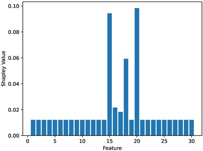
In Fig. 2 we can see the individual Shapley values. The careful observation here is that the Shapley value that shows an increased value is obtained when the empirical distribution value substitutes the original value. This requires further investigation and we leave it for future work. The values that are close to $0.1$ are the values sampled to obtain the original value since it is larger than the empirical distribution value.

Fig. 1Potential function of the execution of the SA

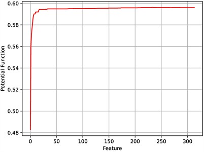
Fig. 2Shapley values of each feature

In this study, we compute the marginal contribution of each feature and, subsequently, the Shapley value for each. Our goal is to demonstrate how Shapley value computation can connect with potential games, specifically illustrating how features’ contributions in a breast cancer dataset can be interpreted in the framework of cooperative game theory. Here, the Shapley value computation is likened to a potential function in a potential game. Each feature’s Shapley value acts as an indicator of how much that feature adds to the potential of the dataset (in terms of predictive accuracy). By connecting Shapley values to potential games, we can view the optimization process as a step toward maximizing this potential function, ensuring that each feature’s role is properly accounted for and optimized within the overall model. Using simulated annealing (SA) for optimization, we dynamically update the Shapley value of each feature to a higher value if a better marginal contribution is identified, which helps prevent the algorithm from becoming trapped in local minima. This dynamic adjustment is key in ensuring the SA process progresses toward an optimal solution in terms of feature contribution, as represented by the potential function.

10. Conclusions

In this article, we deeply explore the Potential Game paradigm, employing it as a structural framework to showcase the inherent interaction between this concept and Shapley values. Through our efforts, a significant connection is unveiled, revealing the profound interrelationship between Shapley values and the fundamental potential function. Additionally, we formulate a gaming scenario wherein the utility functions of individual players stem from their distinct marginal contributions. This intricately crafted game is subsequently subjected to rigorous analysis, confirming its alignment with the essential characteristics of a potential game. As the culmination of our study, we present a discovery: the price of stability for this specific game is solidly established at a value of 1.