Abstract
Accurately analysing features in infrared images of equipment is one of the current directions in the field of power equipment detection and identification. Because infrared images of power equipment have poor resolution, low contrast, and visual blurring problems, this work proposes the use of the squirrel search algorithm to optimize the detection strategy of YOLOv5. First, due to the shortcomings of the squirrel search algorithm, which easily falls into local optima and has a slow convergence speed, in this work, the Henon Consine Seagull search algorithm (HCSSA) is proposed; this algorithm uses Henon chaotic mapping for population initialization and optimizes the predator probability based on the cosine function to improve the algorithm's performance. Second, in the YOLOv5 model, CSP_Faster is used for feature information recognition and to reduce the computational burden, the SKNet mechanism is introduced to ensure the integrity of the image feature information, the SIoU loss function in target classification is used to obtain a better classification effect, and finally, the HCSSA algorithm is optimized for the two hyperparameters of the YOLOv5 model, which are the learning rate and the weight decay. In the simulation experiments, the recognition effect of the proposed algorithm is improved by 8.87 %, 7.67 % and 5.11 % compared with those of YOLOv3, YOLOv4, and YOLOv5, respectively, which shows that the model has a better target detection effect.
1. Introduction
Computer vision, as one of the important directions in the field of deep learning, is receiving increasing attention from researchers. Target recognition is an important component of computer vision, which focuses on accurately finding the target information from the content of a given image or video and is currently applied primarily in the fields of transportation applications [1-2], equipment operation [3], and medical image processing [4-5]. Power equipment is an important component of a power system, and there is an inseparable relationship between its normal operation and the entire power grid. Due to the unpredictability of the occurrence of equipment failure, the development of methods for accurately and quickly detecting and identifying the equipment failure state has become an important research direction. At present, the infrared image recognition method for equipment fault detection is widely used because it is noncontact, fast and safe [6]. However, this method is subject to interference from artificial factors, especially when the image itself has poor resolution and low contrast, and the appearance of visual blurring can easily lead to a reduction in the accuracy of detection. Although scholars have attempted to make some technical improvements [7-10], these algorithms have high complexity themselves, which increases the difficulty of image analysis and detection.
With the rapid development of digital technology, the mutual integration of artificial intelligence technology and image processing technology has become the main direction of current research [11]. In recent years, YOLO [12] has emerged as an excellent target detection algorithm that applies the idea of regression to border localization and object category attribute judgement, reduces the complexity of candidate box extraction, and greatly accelerates the speed of detection. In addition, there are different versions of the YOLO model [13], indicating that it has broader application prospects [14]. However, the YOLO model also suffers from the problem that the model performance is easily degraded by background misdetection and that small targets are easily missed. Equipment fault diagnosis for power systems relies mainly on the observation and identification of infrared images of power equipment to determine whether there is a possibility of equipment failure; however, infrared images of power equipment are easily affected by the influences of temperature and light, which reduce the recognition accuracy. To better detect targets in infrared images of power equipment, the YOLOv5 model was chosen, as it strikes a good balance between model size and accuracy and has a fast training speed, high accuracy, and a relatively simple structure for target detection when compared to the many YOLO versions applied to target characterization. Additionally, based on the properties of the relevant metaheuristic algorithms in [15], this work proposes the optimization of the model parameters with the use of metaheuristic algorithms to improve the recognition performance of the model. In recent years, the sparrow search algorithm [16] has been widely used in various fields due to its advantages, which include a fast convergence speed, simple parameter settings and a simple algorithm structure. Based on the above considerations, this work proposes a power equipment fault diagnosis strategy based on the YOLOv5 neural network with SSA optimization to help power enterprises quickly identify faults in power equipment. The primary contributions of this research are as follows:
1) With respect to the characteristics of power equipment with different volume sizes and shapes, YOLOv5 is used for infrared image recognition and is able to extract features from power equipment images in extreme and complex weather.
2) Due to the shortcomings of the SSA algorithm, which easily falls into local optima and slowly converges, Henon chaotic mapping perturbation is chosen for population initialization, and predator probability optimization based on the cosine function is used to improve the performance of the algorithm.
3) In the current YOLOv5 model, the CSP module is replaced with CSP_Faster, the SKNet attention mechanism is introduced to ensure the completeness of the image feature information, and the SIoU loss function is used in the target classification to obtain better classification results.
4) Simulation experiments illustrate that our proposed algorithm exhibits a significant performance improvement over YOLOv3, YOLOv4, and YOLOv5.
The remainder of this paper is organized as follows: Section 2 describes the current state of research on target detection; Section 3 describes the SSA and YOLOv5 used in this paper; Section 4 describes the YOLOv5 model optimized based on the SSA; Section 5 describes the simulation experiments conducted on the model proposed in this paper, which are used to validate its effectiveness; and Section 6 concludes the paper.
2. Related work
Image target detection methods include traditional methods and deep learning-based methods. The former includes a priori knowledge, template matching and manual feature detection methods, while the latter includes candidate region-based methods and regression-based methods.
2.1. Traditional target detection algorithms
2.1.1. A priori knowledge-based approach
Relying on expert experience, the geometric characteristics of the target and the contextual connection between the target and the background for reasoning, the detection effect is evaluated through the representation and inference of a priori knowledge and the construction of a new knowledge rule base. The judgement process of the a priori knowledge-based method is relatively repetitive and easily influenced by individuals, and the judgement time is long; therefore, this approach cannot provide timely feedback on the detection results.
2.1.2. Method based on template matching
The method is implemented in two steps: First, a template image for each category is constructed via manual design or is learned from the dataset. Then, the template image is superimposed on the given image, the degree of difference between all of the regions in the original image where the target is likely to appear and the template image is calculated, and the degree of difference is used as a metric to determine the location of the target. For example, Leninisha et al. [17] proposed a geometrically deformable model based on width and colour for extracting traffic road information from images. Han [18] et al. used additional information provided by a visual sensor system to improve the reliability of template matching, and experiments illustrated the effectiveness of the method. The template matching-based method has simple steps, but it is too dependent on the template used for detection, is not suitable for detecting multicategory targets, and has poor robustness.
2.1.3. Methods based on manual features
This method involves three steps: First, the candidate region is obtained, and the region in the image where the target may exist is initially located. Due to the uncertainty of the location, shape and size of the target appearing in the image, the sliding window algorithm is usually used to obtain the corresponding region of the target. A representative method is selective search (SS), which combines small-scale regions with similar features into large-scale regions with similar features, which are then merged into a large-scale region, thus obtaining an object image with consistent internal features and a high recall rate [19]. The second is feature extraction, i.e., using manually designed target feature description algorithms to extract local features from selected candidate regions, among which the more typical feature descriptors are HOG (Histogram of Oriented Gradient) [20] and SIFT (scale-invariant feature transform) [21]. In the third step, classification and localization, the features extracted from the candidate region are classified and judged by classifiers, where the commonly used classification algorithms are SVM [22], random forest [23] and various cascade classifiers [24]. Finally, the final target of interest is obtained via non-maximum suppression of the overlapping target candidate frames. Manual feature-based target detection methods can meet the needs of natural image target detection to a certain extent, but due to the difficulty of using manually designed features to express the high-dimensional semantic information of an image, they suffer from the problems of weak generalisability and weak robustness in target detection.
2.2. Deep learning-based target detection algorithm
Deep learning-based target detection methods automatically extract features through DCNNs, do not rely excessively on expert knowledge, and have strong mobility and robustness. The methods can be divided into candidate region-based methods and regression-based methods.
2.2.1. Candidate region-based method
This method focuses on feature selection of candidate regions; this process is based mainly on the CNN algorithm, which divides the detection process into two parts. In the first part, the candidate regions that may contain the target are extracted from the image, and in the second part, the candidate regions are corrected and classified to obtain the desired result. Girshick [25] proposed the Fast-CNN method, which is based on the CNN, but its computational complexity is excessive. He et al. [26] proposed Faster R-CNN, which uses a region-generating network to obtain candidate frames from feature maps and completes all of the steps of target detection in a single deep network, applying the detection mode from the input image directly to the output result. Dai [27] used a fully convolutional neural network for application to Faster R-CNN; in this approach the individual categories are evaluated via location-sensitive feature maps to obtain the corresponding category probability, which accelerates the speed of network detection while ensuring the accuracy of positioning.
2.2.2. Regression-based methods
These methods do not need to generate candidate frames but directly extract the features in the image to predict the target’s category and location information; the representative methods are YOLO and SSD. In YOLO, Zhao [28] proposed the use of clustering method to estimate the prediction bounding box of the target on the basis of YOLOv3, and used Markov chain to determine the distance between the initial cluster and each candidate point, and simulation experiments illustrated that the algorithm has a significant performance improvement. Xiong [29] used background subtraction combined with YOLO to obtain the locations and features of small dynamic targets, and the results revealed that the algorithm has good accuracy and low recall. Zhai [30] proposed a trainable Spiking-YOLO for low-latency and high-performance target detection, and the simulation results revealed that this algorithm has low latency and recall, high performance and detection, and significantly improved precision. Wu [31] proposed the YOLO object detection algorithm based on complex environments, which performs well on mAP values. Zakria [32] and others used a single-stage deep learning target detection model to study an improved YOLOv4 algorithm, and the results revealed improved target detection accuracy and robustness. Luo [33] proposed the YOLOv5-Aircraft method based on the YOLOv5 network, finding that the algorithm can improve the accuracy and speed of target detection, and Xu [34] added a small-scale detection layer, a bottleneck transformer and a CBAM mechanism to the YOLOv7 structure to improve the small-scale target capability of the model. Furthermore, related studies have been conducted on YOLOv8 [35-37]. The above findings indicate that the YOLO family of algorithms constitutes a relatively classical algorithm in the field of target detection, which is prone to reduced target localisation accuracy due to the lack of a priori information when predicting the target position. This phenomenon is due mainly to the lack of the key step of region sampling, which leads to less satisfactory results when detecting images with small targets. In terms of the SSD, Gong [38] proposed the enhanced SSD (FCR-SSD) based on feature cross-strengthening, and simulation experiments revealed that it has high accuracy and good detection speed in the small target detection task. Zhai [39] proposed the DF-SSD algorithm, which uses DenseNet-S-32-1 instead of VGG-16, and introduces a multiscale feature-layer fusion mechanism. The experimental results show that the method has higher detection results for small objects and objects with specific relationships. Huo [40] proposed an SSD algorithm for small object detection based on self-attention combined with feature fusion-SAFF-SSD, and simulation experiments revealed that the method produces good detection results. The above findings indicate that the SSD algorithm independently inputs the image features extracted from different convolutional layers into the corresponding network detection branches, which tends to cause repeated detection, leading to poor detection of small targets in images.
3. Basic algorithms
3.1. Squirrel search algorithm
The squirrel search algorithm [16] is a new swarm intelligence optimization algorithm proposed by Indian scholar Mohit Jain in 2019; it mainly simulates the dynamic gluttony strategy and gliding action of southern squirrels. Compared with existing swarm intelligence optimization algorithms, the algorithm is characterized by greater search efficiency and a simple algorithm structure. This approach requires the following assumptions: there are n squirrels and n trees in the forest, and each squirrel stays on one tree; there are only three types of trees in the forest, i.e., hickory trees, oak trees, and common trees. Among them, hickory and oak trees are food sources, and common trees have no food. There is only one hickory tree NFS, one oak tree (NFS∈(1,n)), and the rest are common trees, and each squirrel searches for food individually and finds the best food source through dynamic foraging behaviour.
Under the above assumptions, the implementation of the SSA is divided into random initializations of the location, fitness ranking and classification, squirrel location updating, seasonal monitoring and random winter relocation.
3.1.1. Random initialization location
The SSA starts with a random initial location. The location of the squirrels is represented by an d-dimensional vector, there are n squirrels in the forest, and the initial location of each squirrel is expressed as follows:
where FSi,j denotes the j(j∈(1,d))-dimensional position of the i(i∈(1,n))th squirrel, U(0,1) denotes a random number between 0 and 1 that follows a uniform distribution, and ubj and lbj denote the upper and lower bounds of the ith squirrel in the j-dimension, respectively.
3.1.2. Adaptation degree ranking and classification
After initializing the position vector for each squirrel, the decision variables are entered into the fitness function, and the resulting fitness value is fs=(fs1,fs2,⋯fsn), where the fitness value for each squirrel is represented as follows:
The fitness value indicates the quality of the food source searched by the squirrels. All of the fitness values are sorted in ascending order via Eq. (3), and the squirrels are categorized according to the sorting results. The squirrel with the smallest fitness value is in the hickory tree FSht, the three squirrels whose fitnesses are sorted between 2-4 are in the oak tree FSat, and the rest of the squirrels are in the common tree FSnt, which are defined in Eq. (4)-(6) as follows:
where index denotes the location of a specific squirrel.
3.1.3. Squirrel location update
Squirrels glide back and forth between different trees in search of food, and this foraging behaviour is affected by the probability Pdp that a predator is present. There are three possible scenarios for squirrel position updating in foraging behaviour:
Scenario 1: Squirrels in Oak Trees Move Towards Hickory Trees.
A squirrel flies from the oak tree towards the hickory tree, and the new position of the squirrel is expressed as follows:
where FStat denotes the position of the squirrel on the oak tree in generation t, FStht denotes the position of the squirrel on the hickory tree in generation t, t denotes the current number of iterations, dg is the sliding distance, Gc is the sliding constant (usually taken as 1.9), R1 is the random number obeying the uniform distribution between (0, 1), and Pdp is 0.1.
Scenario 2: Squirrels in Common Trees Move Towards Oak Trees.
A squirrel flies from the normal tree towards the oak tree, and the new position of the squirrel is expressed as follows:
where FStnt denotes the position of the squirrel on the common tree in generation t and where R2 is a random number that obeys a uniform distribution between (0, 1).
Scenario 3: Squirrels in Common Trees Move Towards Hickory Trees.
A squirrel flies from the normal tree towards the hickory tree, and the new position of the squirrel is expressed as follows:
where R3 is a random number that obeys a uniform distribution between (0, 1).
3.1.4. Seasonal monitoring and random winter relocation
The foraging behaviour of squirrels is strongly influenced by the season. Compared with frequent activities in summer, in mid-winter, squirrels are less active to conserve energy, leading to stagnation. Seasonal monitoring is thus introduced into the algorithm to prevent the algorithm from falling into local optima, and the number of seasons is calculated as follows:
The minimum value of the seasonal constant is as follows:
where t and tmax denote the current iteration number and the maximum iteration number, respectively. When Stc<Smin, the winter season is over, and Eq. (12) is used to randomly locate the position of the squirrels in the common tree who cannot find food:
levy' flight is a mathematical tool for enhancing the global optimization algorithm, which can cause the population to evolve away from or avoid falling into local optima. In this algorithm, levy'(n) is expressed as follows:
where ra and rb obey a normal uniformly distributed random number between (0, 1) and β is 1.5:
where Γ(x)=(x-1)!
3.2. YOLOv5 model
YOLOv5 is a single-stage target detection algorithm that divides input images into countless regions by using a single convolutional neural network and calculates each region class probability and target frame. It contains four primary components: the input, backbone, neck and output.
3.2.1. Input side
This component mainly consists of three parts. The first part is mosaic data enhancement, that is, random scaling, cropping, lining up and splicing of images, which can improve the robustness of the detection model. In the second part of the adaptive anchor frame calculation, the initial anchor frame is set before training, and an inverse update of the model parameters is completed according to comparison with the real frame during training. In the third part of adaptive image scaling, i.e., when the letterbox function is improved, by calculating the most suitable image size, the image features are better preserved, and the detection speed is improved.
3.2.2. Backbone
The backbone is the main part of the YOLOv5 model. It primarily extracts the feature information from the target area, and it uses CSPDarknet as the backbone, which aims to fully extract the target feature information in the detection area through the Focus and CSP structure to improve the detection performance of the whole model.
3.2.3. Neck
The neck structure makes full use of the target feature information extracted by the backbone network in the detection area and further performs weighted fusion of this feature information and processing; finally, the output results are classified and localized by the output.
3.2.4. Output
The output is responsible for classifying and predicting the feature information extracted from the target area in the backbone network after compression and fusion by the neck. The network uses 3 sets of 1×1 convolutional structures with output feature mappings of 76×76, 38×38 and 19×19. Each detection layer finally outputs a 30-channel vector.
4. YOLOv5 model based on SSA optimization
To further improve the detection performance of the YOLOv5 model for image targets, we first improved the structure of YOLOv5 and then optimized its parameters by using the improved SSA algorithm to increase the overall performance.
4.1. Improved YOLOv5 model
4.1.1. CSP module optimization
The backbone network of the YOLOv5 architecture consists of several CSP modules. This module mainly reduces the computational cost and memory usage during network training and maintains the performance of the model. By dividing the feature map into two parts and processing them independently at different stages, the number of computations can be reduced, and the accuracy and precision of the model can be improved; however, due to the large number of parameters in the convolutional kernel of the module, a large number of computations are needed to detect the target. On this basis, the design of the Faster Net network structure inspired the optimization of the CSP module, and this work proposes the CSP_Faster module instead of CSP1_1, CSP1_2 and CSP1_3. In this module, to maintain consistency in terms of the number of channels in the output feature map and the ordinary convolution operation, the point-by-point convolution operation is attached to the local convolution, which can pay more attention to the centre of the image, thus reducing the amount of computation. The improved CSP_Faster structure is shown in Fig. 1.
Fig. 1CSP_Faster structure

4.1.2. Introduction of the SKNet attention mechanism
In the traditional convolutional neural network, the size of the convolutional kernel is not consistent, so it cannot effectively capture the image features of different scales; therefore, the SKNet attention mechanism is incorporated in the YOLOv5 model, and a mechanism is introduced into the last layer of the backbone to connect it with the neck. This connection can ensure the completeness of the information of the image features and can improve the feature information expression ability of the graph, as shown in Fig. 2.
Fig. 2SKNet attention mechanism

4.1.3. Using the SIoU loss function
A problem in target detection is that the background in which the target image is located is complex and generates more false detection frames. Therefore, the SIoU function, which introduces the vector angle between the real and predicted frames and redefines the correlation damage function, can effectively reduce the total degrees of freedom of the loss and improve the training speed and accuracy. A description of the relevant parameters is provided in the [41].
4.2. Improved SSA
The SSA has the advantages of strong global search ability and adaptive ability, but like most metaheuristic algorithms, the algorithm is prone to falling into local optima as the number of iterations continues to increase, resulting in lower convergence performance. To further improve the performance of this algorithm, it was optimized to different degrees from two aspects: population initialization and cosine-based migration behaviour.
4.2.1. Henon chaos-based initialization
The squirrel search algorithm generates initialized populations randomly in the search space, which cannot traverse the search space uniformly, resulting in some limitations in the search range. To solve this problem, the algorithm is optimized by using the improved Henon chaos algorithm, which has better uniformity and faster iteration speeds than a single chaotic mapping. The formula is as follows:
where a and b are the parameters.
4.2.2. Predator probability optimization
In the process of updating the positions of individual squirrels, the predator probability A causes the squirrels to use different search strategies. In the early stage of the algorithm, a global search is needed to expand the whole solution space, and in the late stage of the algorithm's optimization search, the individual squirrels tend to gather near the optimal solution, which causes the algorithm to fall into a local optimum; therefore, more local development of the algorithm is needed. To address this issue, an adaptive optimization strategy is adopted to optimize the predator probability B according to Eq. (16), which can ensure that C is able to find a balance between the global search and local exploitation of the algorithm as the number of iterations increases:
where Pmax and Pmin are the maximum and minimum values of predator probability, respectively, and where tmax is the maximum number of iterations.
4.3. Complexity analysis
The time complexity of the algorithm is related mainly to the number of individuals in the population, the maximum number of iterations, and the problem dimension. When initializing the population position, the time complexity is approximately O (number of squirrels × number of dimensions). During the iterative process, each iteration traverses all of the individuals for the fitness calculation, position update and other operations, and its time complexity is O (maximum number of iterations × number of squirrels × number of dimensions). Taken together, the time complexity of the whole algorithm is usually on the order of O (maximum number of iterations × number of squirrels × number of dimensions).
The space complexity of the algorithm primarily depends on the storage of information related to the individuals within the population, as it is necessary to store information such as the position of each individual squirrel (corresponding to the population individuals), the optimal position of the individual, and the optimal value. Since there are a number of individual squirrels in the population and each individual involves the number of dimensions, the space complexity is roughly of the order of O (the number of squirrels × the number of dimensions).
4.4. Optimizing the YOLOv5 model based on the SSA
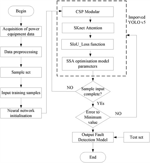
The 2 hyperparameters, the learning rate and weight decay, are among the most important components that affect the performance of YOLOv5; therefore, the SSA is used to optimize the model parameters, and the specific steps are as follows:
Step 1: Define the objective function. The image accuracy of the YOLOv5 model is set as the objective function of the SSA algorithm.
Step 2: Initialize the squirrel individuals. Each squirrel individual is represented as a set of parameters consisting of the learning rate and weight decay parameters.
Step 3: Set the fitness function. According to each squirrel individual, calculate the model performance metric (classification accuracy) as the fitness function of the individual.
Step 4: Set the individual position as the current population optimal position.
Step 5: Perform population initialization and predator probability optimization.
Step 6: Execute the locomotor migration behaviour.
Step 7: Perform aggressive behaviour.
Step 8: Update the global optimal solution. The individual squirrel with the highest fitness is selected as the global optimal solution.
Step 9: Iterative update: Repeat Steps 6 to 7 until a preset stopping condition is reached, such as when the maximum number of iterations is reached or the target accuracy rate is reached.
Step 8: Output the optimal solution. The neural network parameter settings corresponding to the global optimal solution, i.e., the best parameters of the optimized YOLOv5 neural network, are output.
The HCSSA-YOLOv5 algorithm is used to perform detection on the infrared images of power equipment in the process shown in Fig. 3.
Fig. 3Flowchart of the algorithm proposed in this paper
5. Simulation experiment
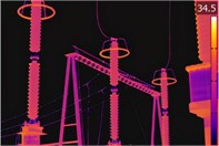
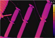
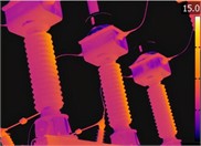
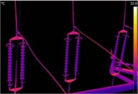
To illustrate the effectiveness of the model proposed in this paper in terms of detecting targets in infrared images of electric power equipment, the simulation environment employed a CPU Core I7, 32 GB of memory, and a hard disk capacity of 2T. The two parts of the experiment proceeded as follows: the first part verified the performance of the HCSSA algorithm proposed in this paper, which was accomplished through the MATLAB 2012 simulation software, and the second part verified the improved algorithmic model for detecting the effect of the selection of the GPU. In this experiment, the selected GPU was the RTX3050, and the Python software programming was also used. The TensorFlow 1.10.0 open-source framework and the Windows 10 operating system were also used. Fig. 4 shows infrared images of commonly used pieces of equipment.
Fig. 4Some commonly used electrical equipment
a) Surge arrester
b) Circuit breakers
c) Transformers
d) Insulators
5.1. HCSSA algorithm performance
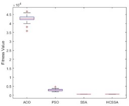
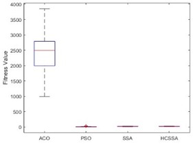
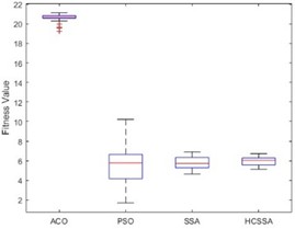
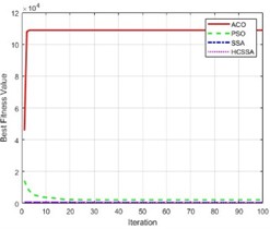
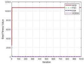
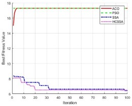
To illustrate the performance of the HCSSA algorithm, the ACO, PSO and SSA were chosen as comparison algorithms and the Ackley function, Step function and Sphere function were chosen as test functions, respectively. The number of iterations of the four algorithms was set to 100, and they were run 30 times. In the ACO algorithm, the number of ants was 50, the pheromone evaporation rate was 0.5, the pheromone factor was 1, the heuristic factor was 2, and the probability was 0.9. In the PSO algorithm, the number of particles was set to 50, the inertia weight was 0.7, and the cognitive coefficient and social coefficient were 1.4. In the SSA algorithm, the number of squirrels was 30, the lower bound was –5, the upper bound was 5, the step factor was 0.1, and the stochastic factor was 0.5. In the HCSSA algorithm, the initial value in the Henon chaotic mapping was 0.1; parameters a and b were 1.4 and 0.3, respectively; the maximum value of the predation probability was 0.8; and the minimum value was 0.2. Table 1 shows the maximum, minimum, average, and standardized values of the four algorithms for the conditions of 2 dimensions, 10 dimensions and 50 dimensions and the standard value comparison results. Fig. 5 presents the box plots of the three benchmarking functions in 100 dimensions, and Fig. 6 shows the optimal fitness value curves for the three benchmark test functions in 100 dimensions. According to the results recorded in Table 2, the HCSSA algorithm has good results in different dimensions in the three test functions, especially in the 2-dimensional condition of the Step function, and both the HCSSA and SSA reach 0. However, in the 5-dimensional and 10-dimensional conditions, the HCSSA has a better metric effect than the SSA does, and the four algorithms in the Ackley function and the Sphere function only obtain a minimum value of 0 in 2 dimensions. In the high-dimensional case, the indicator results for the ACO and PSO algorithms are not as good as those of the SSA and HCSSA, and the HCSSA has a more obvious advantage over the SSA, which shows that the performance effect of the HCSSA algorithm is obvious. The results shown in Fig. 5 indicate that the ACO algorithm is in a higher position in all three functions, which indicates that the optimal solution to the algorithm is relatively poor. In the Step function, the ACO algorithm has a wider box, while the PSO, SSA and HCSSA algorithms have a smaller box and lower position. The SSA and HCSSA algorithms present the smallest boxes, which indicates that the SSA and HCSSA algorithms are more stable. In the Sphere function, the ACO algorithm has wider boxes, whereas the other three algorithms have exceptionally narrow boxes, which also indicates that the PSO, SSA and HCSSA algorithms are stable in terms of the Sphere function. The PSO algorithm has wider boxes in the Ackley function, and the ACO, SSA and HCSSA algorithms have narrower boxes, but the HCSSA algorithm is even narrower, which indicates that the HCSSA algorithm is very stable. According to the results shown in Fig. 6, the ACO algorithm has the weakest optimal value for all three test functions, whereas the SSA and HCSSA have better advantages over the PSO, especially for the Ackley function. The HCSSA algorithm obtains the optimal solution due to the other three algorithms.
Table 1Comparison of the metrics of the four algorithms on three benchmark functions
Test function | Algorithm | DIM | Max-value | Min-value | Ave-value | Std-value |
Ackley | ACO | 2 | 21.5703 | 16.0409 | 21.4883 | 0.5902 |
10 | 21.5703 | 20.7074 | 21.5557 | 0.0978 | ||
50 | 21.5703 | 21.1165 | 21.5636 | 0.0474 | ||
PSO | 2 | 12.7432 | 0 | 0.4731 | 1.9324 | |
10 | 19.8277 | 5.0897 | 6.3206 | 2.6953 | ||
50 | 20.0060 | 15.7413 | 16.0748 | 0.7579 | ||
SSA | 2 | 1.0153 | 0.0160 | 0.2830 | 0.2124 | |
10 | 7.6349 | 4.7038 | 6.5071 | 0.7507 | ||
50 | 9.8280 | 8.9490 | 9.4833 | 0.2222 | ||
HCSSA | 2 | 2.5228 | 0.0285 | 0.9124 | 0.6139 | |
10 | 3.6634 | 2.5651 | 3.2911 | 0.2860 | ||
50 | 3.7065 | 3.4891 | 3.6434 | 0.0551 | ||
Sphere | ACO | 2 | 2147.4836 | 74.4132 | 2118.9259 | 220.8498 |
10 | 10737.4182 | 3037.9726 | 10658.9750 | 769.9345 | ||
50 | 53687.0912 | 17603.7898 | 53326.2582 | 3608.3301 | ||
PSO | 2 | 2.0332 | 0.0000 | 0.0672 | 0.3486 | |
10 | 663.8604 | 0.0211 | 13.1938 | 71.5154 | ||
50 | 7484.7075 | 706.0328 | 1017.6451 | 1015.1604 | ||
SSA | 2 | 0.0416 | 0.0006 | 0.0091 | 0.0104 | |
10 | 24.9005 | 8.1003 | 14.6762 | 3.9213 | ||
50 | 252.9942 | 211.6295 | 234.0806 | 11.8494 | ||
HCSSA | 2 | 0.5709 | 0.0006 | 0.0451 | 0.1032 | |
10 | 28.2985 | 8.8187 | 18.0450 | 4.9776 | ||
50 | 271.0158 | 186.4901 | 233.2787 | 18.1956 | ||
Step | ACO | 2 | 2178.0000 | 180.0000 | 2150.3700 | 213.2217 |
10 | 10890.0000 | 3001.0000 | 10811.1100 | 788.9000 | ||
50 | 54450.0000 | 19562.0000 | 54101.1200 | 3488.8000 | ||
PSO | 2 | 29.0000 | 0 | 0.5300 | 3.3798 | |
10 | 1236.0000 | 39.0000 | 78.6200 | 166.1495 | ||
50 | 6488.0000 | 1034.0000 | 1249.0600 | 739.8844 | ||
SSA | 2 | 0 | 0 | 0 | 0 | |
10 | 22.0000 | 9.0000 | 15.4333 | 4.1745 | ||
50 | 272.0000 | 202.0000 | 248.4000 | 15.8802 | ||
HCSSA | 2 | 0 | 0 | 0 | 0 | |
10 | 24.0000 | 6.0000 | 16.8000 | 3.6141 | ||
50 | 252.0000 | 160.0000 | 227.3000 | 22.4717 |
To illustrate the performance of the HCSSA algorithm, four improved algorithms, the SSA, DSSA [42], HSSA [43], and ASSA [44], were chosen as the comparison algorithms in this work. Under 100-dimensional conditions, the tests were conducted using the above three benchmark functions, and the curve changes in the fitness values of the four algorithms are shown in Fig. 7. The results in the figure indicate that with the gradual increase in the number of iterations, the fitness function values of the four algorithms exhibit a decreasing trend compared with those of the SSA, DSSA, HSSA, and ASSA, whereas the HCSSA algorithm has smaller fitness function values, illustrating the good performance of the algorithms.
Fig. 5Box plots of the four algorithms
a) Step function
b) Sphere function
c) Ackley function
Fig. 6Fitness values of the four algorithms
a) Step function
b) Sphere function
c) Ackley function
Fig. 7Fitness values of the five algorithms
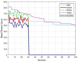
a) Step function
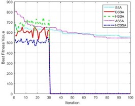
b) Sphere function
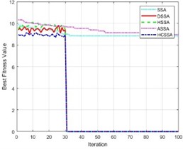
c) Ackley function
5.2. HCSSA-IYOLOv5 model target detection performance
To further illustrate that the algorithms proposed in this paper have good detection performance, two ablation experiments and different scene experiments were conducted to compare the three different improved YOLOv3 [31], YOLOv4 [32], and YOLOv5 [33] algorithms the HCSSA algorithm. Moreover, the recall rate (R) and precision rate (P) were used as discriminative methods of model accuracy, and their respective formulas are as follows:
where, Tp and Fp denote the number of correctly identified positive and negative samples, respectively; Fn denotes the number of positive samples misclassified as negative; and n denotes the number of all samples labelled as positive.
5.2.1. Ablation experiment
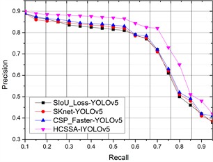
To further illustrate the effect of the improved measures on the performance of the algorithms, the three improved measures for YOLOv5 were compared with HCSSA-IYOLOv5, and the results of the comparison are shown in Fig. 8. The figure shows that the P value of all four algorithms gradually decreases with increasing R value, but the P value of HCSSA-IYOLOv5 is better than the results of the other three improvement measures, which indicates that the algorithm proposed in this paper has better performance.
Fig. 8Comparative results of the ablation experiments
5.2.2. Experimental comparison of different scenes
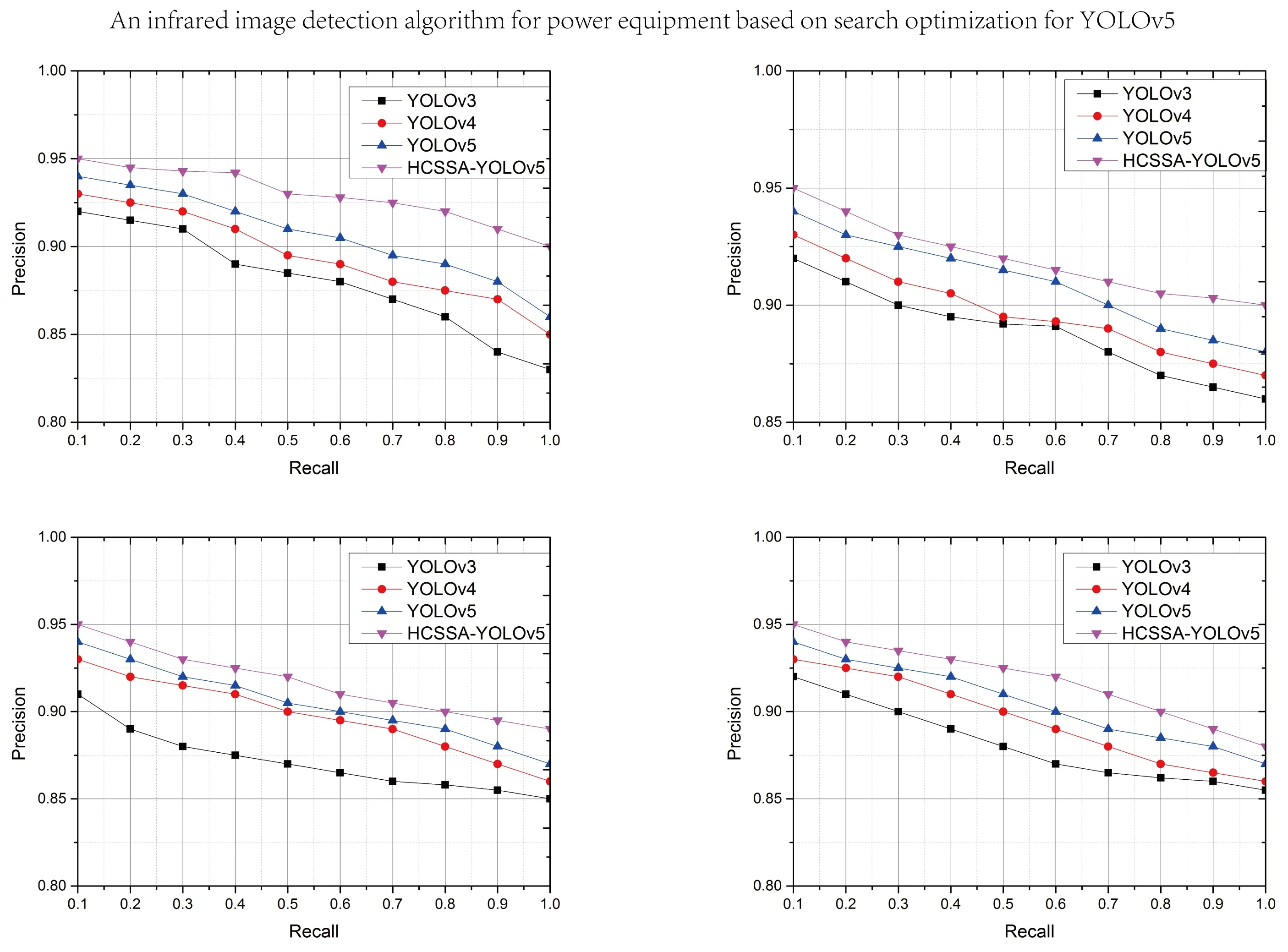
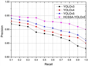
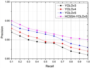
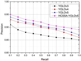
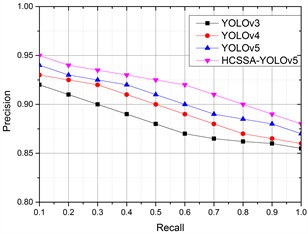
To further illustrate the recognition effect of the algorithms on infrared images in different weather conditions (heavy rain, lightning, gusty wind, and hail), the lightning arrester infrared image was chosen as the research object, and the PR results of the four algorithms are shown in Fig. 9.
Fig. 9PRs of the four algorithms in different scenarios
a) Heavy rain
b) Lightning
c) Gusty wind
d) Hail
According to the detection results, in four different scenarios, the corresponding PR values of our proposed algorithms have better results than the other three improved YOLO algorithms, which have better application results, illustrating that CSP_Faster improves feature information recognition, the SKNet mechanism ensures the integrity of the image feature information, and the SIoU loss function obtains better classification results. After the optimization of the SSA algorithm, the model’s performance improves, and the feature acquisition ability of infrared images is obviously enhanced.
5.2.3. Comparison of the recognition time
To further illustrate the performance of this algorithm, we collected 100 infrared images of four kinds of power equipment in different scenes to compare the recognition time of the four algorithms, and the results are shown in Table 2. The results in the table indicate that these algorithms have different results in terms of the power equipment recognition time, but the advantages of the proposed algorithm are more obvious. When detecting targets in images of surge arresters, compared with those of the YOLOv3, YOLOv4, and YOLOv5, the recognition rates increased by 2.95 %, 2.61 % and 1.85 %, respectively. Furthermore, the recognition rates for circuit breakers increased by 6.49 %, 5.61 % and 2.54 %, respectively; the recognition rates for mutual inductors increased by 3.07 %, 2.63 % and 1.95 %, respectively; and the recognition rates for the insulator improved by 2.13 %, 1.94 % and 1.32 %, respectively. These results indicate that the optimization of the CSP module, the introduction of the SKNet attention mechanism and the use of the SIoU loss function in the YOLOv5 model increase the performance of the model and thus reduce the identification time.
Table 2Comparison of the time consumed by the algorithms while identifying four types of power devices
Algorithm | Surge arrester (S) | Circuit breakers (S) | Transformers (S) | Insulators (S) |
YOLOv3 | 12.21 | 15.92 | 16.43 | 16.26 |
YOLOv4 | 12.17 | 15.79 | 16.36 | 16.23 |
YOLOv5 | 12.08 | 15.33 | 16.25 | 16.13 |
HCSSA-IYOLOv5 | 11.86 | 14.95 | 15.94 | 15.92 |
5.2.4. Comparison of detection target effects
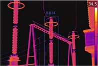
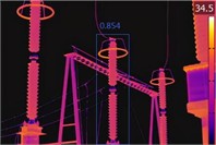
Figs. 10-13 present the results of the target detection experiments for the four algorithms on infrared images of the four devices. Fig. 10 shows the lightning arrester detection results; the YOLOv3 detection result is 0.821, the YOLOv4 detection result is 0.834, the YOLOv5 detection result is 0.854, and the ISOA-IYOLOv5 detection result is 0.893.
Fig. 10Recognition by the four algorithms on surge arrester infrared images

a) YOLOv3
b) YOLOv4
c) YOLOv5

d) HCSSA-IYOLOv5
Fig. 11Recognition by the four algorithms on infrared images of circuit breakers
a) YOLOv3
b) YOLOv4
c) YOLOv5
d) HCSSA-IYOLOv5
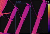
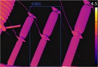
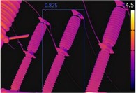
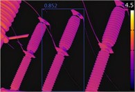
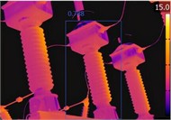
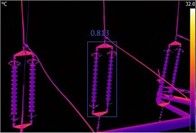
Fig. 11 shows the circuit breaker detection results; the YOLOv3 detection result is 0.794, the YOLOv4 detection result is 0.801, the YOLOv5 detection result is 0.825, and the HCSSA-IYOLOv5 detection result is 0.852. The detection results of the transformer are shown in Fig. 12, where the YOLOv3 detection result is 0.788, the YOLOv4 detection result is 0.793, the YOLOv5 detection result is 0.815, and the HCSSA-IYOLOv5 detection result is 0.863. In Fig. 13, the insulator detection results are shown, and the YOLOv3 detection result is 0.812, the YOLOv4 detection result is 0.823, the YOLOv5 detection result is 0.834, and the HCSSA-IYOLOv5 detection result is 0.892. According to the above detection results, the HCSSA-IYOLOv5 algorithm proposed in this paper outperforms YOLOv3, YOLOv4, and YOLOv5 by 8.87 %, 7.67 %, and 5.11 %, respectively, on average. These results show that the algorithm has good target detection and recognition effects.
Fig. 12Recognition by the four algorithms on infrared images of transformers
a) YOLOv3

b) YOLOv4

c) YOLOv5

d) HCSSA-IYOLOv5
Fig. 13Recognition by the four algorithms on insulator infrared images

a) YOLOv3
b) YOLOv4
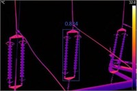
c) YOLOv5
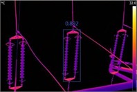
d) HCSSA-IYOLOv5
6. Conclusions
This work proposes the HCSSA-IYOLOv5 target detection algorithm. Simulation experiments illustrate the detection effect of the algorithm, but because power equipment is affected by the complexity of the natural environment, the existence of defects, information transmission, and other delays and problems, the algorithm’s recognition effect is lower than it could be, which is an important research direction. In the near future, with the optimization and quantization of the YOLOv5 model, the recognition accuracy and computational efficiency will continue to improve, adapting to the diversity and complexity of different power equipment. Thus, more intelligent and automated equipment inspection and fault detection can be realized, and the operation and maintenance efficiency and safety of electric power facilities can be improved.
References
-
C. H. Bahnsen and T. B. Moeslund, “Rain removal in traffic surveillance: does it matter?,” IEEE Transactions on Intelligent Transportation Systems, Vol. 20, No. 8, pp. 2802–2819, Aug. 2019, https://doi.org/10.1109/tits.2018.2872502
-
Y. Han and D. Hu, “Multispectral fusion approach for traffic target detection in bad weather,” Algorithms, Vol. 13, No. 11, p. 271, Oct. 2020, https://doi.org/10.3390/a13110271
-
A. Lauricella, J. Cannon, S. Branting, and E. Hammer, “Semi-automated detection of looting in Afghanistan using multispectral imagery and principal component analysis,” Antiquity, Vol. 91, No. 359, pp. 1344–1355, Sep. 2017, https://doi.org/10.15184/aqy.2017.90
-
K. Jnawali, B. Chinni, V. Dogra, and N. Rao, “Automatic cancer tissue detection using multispectral photoacoustic imaging,” International Journal of Computer Assisted Radiology and Surgery, Vol. 15, No. 2, pp. 309–320, Dec. 2019, https://doi.org/10.1007/s11548-019-02101-1
-
O. Özkaraca et al., “Multiple brain tumor classification with dense CNN architecture using brain MRI images,” Life, Vol. 13, No. 2, p. 349, Jan. 2023, https://doi.org/10.3390/life13020349
-
C. Xia et al., “Infrared thermography‐based diagnostics on power equipment: State‐of‐the‐art,” High Voltage, Vol. 6, No. 3, pp. 387–407, Nov. 2020, https://doi.org/10.1049/hve2.12023
-
A. S. N. Huda and S. Taib, “Application of infrared thermography for predictive/preventive maintenance of thermal defect in electrical equipment,” Applied Thermal Engineering, Vol. 61, No. 2, pp. 220–227, Nov. 2013, https://doi.org/10.1016/j.applthermaleng.2013.07.028
-
Y. Laib Dit Leksir, M. Mansour, and A. Moussaoui, “Localization of thermal anomalies in electrical equipment using infrared thermography and support vector machine,” Infrared Physics and Technology, Vol. 89, pp. 120–128, Mar. 2018, https://doi.org/10.1016/j.infrared.2017.12.015
-
C. Shanmugam and E. Chandira Sekaran, “IRT image segmentation and enhancement using FCM-MALO approach,” Infrared Physics and Technology, Vol. 97, pp. 187–196, Mar. 2019, https://doi.org/10.1016/j.infrared.2018.12.032
-
M. P. Manda, C. Park, B. Oh, and H.-S. Kim, “Marker-based watershed algorithm for segmentation of the infrared images,” in International SoC Design Conference (ISOCC), pp. 227–228, Oct. 2019, https://doi.org/10.1109/isocc47750.2019.9027721
-
N. M. Nasrabadi, “Hyperspectral target detection: an overview of current and future challenges,” IEEE Signal Processing Magazine, Vol. 31, No. 1, pp. 34–44, Jan. 2014, https://doi.org/10.1109/msp.2013.2278992
-
J. Redmon, S. Divvala, R. Girshick, and A. Farhadi, “You only look once: unified, real-time object detection,” in IEEE Conference on Computer Vision and Pattern Recognition (CVPR), pp. 779–788, Jun. 2016, https://doi.org/10.1109/cvpr.2016.91
-
P. Jiang, D. Ergu, F. Liu, Y. Cai, and B. Ma, “A review of Yolo algorithm developments,” Procedia Computer Science, Vol. 199, pp. 1066–1073, Jan. 2022, https://doi.org/10.1016/j.procs.2022.01.135
-
T. Diwan, G. Anirudh, and J. V. Tembhurne, “Object detection using YOLO: challenges, architectural successors, datasets and applications,” Multimedia Tools and Applications, Vol. 82, No. 6, pp. 9243–9275, Aug. 2022, https://doi.org/10.1007/s11042-022-13644-y
-
D. H. Wolpert and W. G. Macready, “No free lunch theorems for optimization,” IEEE Transactions on Evolutionary Computation, Vol. 1, No. 1, pp. 67–82, Apr. 1997, https://doi.org/10.1109/4235.585893
-
M. Jain, V. Singh, and A. Rani, “A novel nature-inspired algorithm for optimization: Squirrel search algorithm,” Swarm and Evolutionary Computation, Vol. 44, pp. 148–175, Feb. 2019, https://doi.org/10.1016/j.swevo.2018.02.013
-
S. Leninisha and K. Vani, “Water flow based geometric active deformable model for road network,” ISPRS Journal of Photogrammetry and Remote Sensing, Vol. 102, pp. 140–147, Apr. 2015, https://doi.org/10.1016/j.isprsjprs.2015.01.013
-
Y. Han, “Reliable template matching for image detection in vision sensor systems,” Sensors, Vol. 21, No. 24, p. 8176, Dec. 2021, https://doi.org/10.3390/s21248176
-
J. R. R. Uijlings, K. E. A. van de Sande, T. Gevers, and A. W. M. Smeulders, “Selective search for object recognition,” International Journal of Computer Vision, Vol. 104, No. 2, pp. 154–171, Apr. 2013, https://doi.org/10.1007/s11263-013-0620-5
-
N. Dalal and B. Triggs, “Histograms of oriented gradients for human detection,” in IEEE Computer Society Conference on Computer Vision and Pattern Recognition (CVPR’05), Vol. 1, pp. 886–893, Nov. 2024, https://doi.org/10.1109/cvpr.2005.177
-
D. G. Lowe, “Distinctive image features from scale-invariant keypoints,” International Journal of Computer Vision, Vol. 60, No. 2, pp. 91–110, Nov. 2004, https://doi.org/10.1023/b:visi.0000029664.99615.94
-
Z. Deng and L. Zhou, “Detection and recognition of traffic planar objects using colorized laser scan and perspective distortion rectification,” IEEE Transactions on Intelligent Transportation Systems, Vol. 19, No. 5, pp. 1485–1495, May 2018, https://doi.org/10.1109/tits.2017.2723902
-
J. L. Speiser, M. E. Miller, J. Tooze, and E. Ip, “A comparison of random forest variable selection methods for classification prediction modeling,” Expert Systems with Applications, Vol. 134, pp. 93–101, Nov. 2019, https://doi.org/10.1016/j.eswa.2019.05.028
-
H. Li, Z. Lin, X. Shen, J. Brandt, and G. Hua, “A convolutional neural network cascade for face detection,” in IEEE Conference on Computer Vision and Pattern Recognition (CVPR), pp. 5325–5334, Jun. 2015, https://doi.org/10.1109/cvpr.2015.7299170
-
R. Girshick, “Fast R-CNN,” in IEEE International Conference on Computer Vision (ICCV), pp. 1107–1115, Dec. 2015, https://doi.org/10.1109/iccv.2015.169
-
S. Ren, K. He, R. Girshick, and J. Sun, “Faster R-CNN: towards real-time object detection with region proposal networks,” IEEE Transactions on Pattern Analysis and Machine Intelligence, Vol. 39, No. 6, pp. 1137–1149, Jun. 2017, https://doi.org/10.1109/tpami.2016.2577031
-
J. Dai, Y. Li, K. He, and J. Sun, “R-fcn: object detection via region-based fully convolutional networks,” in 30th Conference on Neural Information Processing Systems (NIPS 2016), 2016.
-
L. Zhao and S. Li, “Object detection algorithm based on improved YOLOv3,” Electronics, Vol. 9, No. 3, p. 537, Mar. 2020, https://doi.org/10.3390/electronics9030537
-
J. Xiong, J. Wu, M. Tang, P. Xiong, Y. Huang, and H. Guo, “Combining YOLO and background subtraction for small dynamic target detection,” The Visual Computer, pp. 1–10, Mar. 2024, https://doi.org/10.1007/s00371-024-03342-1
-
M. Yuan, C. Zhang, Z. Wang, H. Liu, G. Pan, and H. Tang, “Trainable Spiking-YOLO for low-latency and high-performance object detection,” Neural Networks, Vol. 172, p. 106092, Apr. 2024, https://doi.org/10.1016/j.neunet.2023.106092
-
W. Wu and J. Lai, “Multi camera localization handover based on YOLO object detection algorithm in complex environments,” IEEE Access, Vol. 12, pp. 15236–15250, Jan. 2024, https://doi.org/10.1109/access.2024.3357519
-
Z. Zakria, J. Deng, R. Kumar, M. S. Khokhar, J. Cai, and J. Kumar, “Multiscale and direction target detecting in remote sensing images via modified YOLO-v4,” IEEE Journal of Selected Topics in Applied Earth Observations and Remote Sensing, Vol. 15, pp. 1039–1048, Jan. 2022, https://doi.org/10.1109/jstars.2022.3140776
-
S. Luo, J. Yu, Y. Xi, and X. Liao, “Aircraft target detection in remote sensing images based on improved YOLOv5,” IEEE Access, Vol. 10, pp. 5184–5192, Jan. 2022, https://doi.org/10.1109/access.2022.3140876
-
S. Xu, Z. Chen, H. Zhang, L. Xue, and H. Su, “Improved remote sensing image target detection based on YOLOv7,” Optoelectronics Letters, Vol. 20, No. 4, pp. 234–242, Mar. 2024, https://doi.org/10.1007/s11801-024-3063-z
-
A. Milanovic, L. Jovanovic, M. Zivkovic, N. Bacanin, M. Cajic, and M. Antonijevic, “Exploring pre-trained model potential for reflective vest real time detection with YOLOv8 models,” in 3rd International Conference on Applied Artificial Intelligence and Computing (ICAAIC), pp. 1210–1216, Jun. 2024, https://doi.org/10.1109/icaaic60222.2024.10575617
-
V. Markovic, J. C. Milovanovic, A. Jokic, L. Jovanovic, M. Zivkovic, and N. Bacanin, “Exploring power line arc detection using YOLOv8 computer vision models,” in 2024 Second International Conference on Intelligent Cyber Physical Systems and Internet of Things (ICoICI), pp. 903–907, Aug. 2024, https://doi.org/10.1109/icoici62503.2024.10696297
-
L. Jovanovic et al., “Computer vision based areal photographic rocket detection using YOLOv8 models,” International Journal of Robotics and Automation Technology, Vol. 11, pp. 37–49, Sep. 2024, https://doi.org/10.31875/2409-9694.2024.11.03
-
L. Gong, X. Huang, Y. Chao, J. Chen, and B. Lei, “An enhanced SSD with feature cross-reinforcement for small-object detection,” Applied Intelligence, Vol. 53, No. 16, pp. 19449–19465, Mar. 2023, https://doi.org/10.1007/s10489-023-04544-1
-
S. Zhai, D. Shang, S. Wang, and S. Dong, “DF-SSD: an improved SSD object detection algorithm based on DenseNet and feature fusion,” IEEE Access, Vol. 8, pp. 24344–24357, Jan. 2020, https://doi.org/10.1109/access.2020.2971026
-
B. Huo, C. Li, J. Zhang, Y. Xue, and Z. Lin, “SAFF-SSD: Self-attention combined feature fusion-based SSD for small object detection in remote sensing,” Remote Sensing, Vol. 15, No. 12, p. 3027, Jun. 2023, https://doi.org/10.3390/rs15123027
-
S. Du, B. Zhang, and P. Zhang, “Scale-sensitive IOU loss: an improved regression loss function in remote sensing object detection,” IEEE Access, Vol. 9, pp. 141258–141272, Jan. 2021, https://doi.org/10.1109/access.2021.3119562
-
B. Jena, M. K. Naik, A. Wunnava, and R. Panda, “A differential squirrel search algorithm,” in Lecture Notes in Networks and Systems, Singapore: Springer Singapore, 2021, pp. 143–152, https://doi.org/10.1007/978-981-16-0695-3_15
-
H. Hu, L. Zhang, Y. Bai, P. Wang, and X. Tan, “A hybrid algorithm based on squirrel search algorithm and invasive weed optimization for optimization,” IEEE Access, Vol. 7, pp. 105652–105668, Jan. 2019, https://doi.org/10.1109/access.2019.2932198
-
Y. Zhang, C. Wei, J. Zhao, Y. Qiang, W. Wu, and Z. Hao, “Adaptive mutation quantum-inspired squirrel search algorithm for global optimization problems,” Alexandria Engineering Journal, Vol. 61, No. 9, pp. 7441–7476, Sep. 2022, https://doi.org/10.1016/j.aej.2021.11.051
About this article
The second batch of teaching reform projects for vocational education in Zhejiang Province during the 14th Five Year Plan period, project No: jg20240238.
The datasets generated during and/or analyzed during the current study are available from the corresponding author on reasonable request.
The authors declare that they have no conflict of interest.

