Unknown input reconstruction in non-linear dynamical systems using homotopy optimization

1. Introduction

The unknown input reconstruction problem deals with unmodelled dynamics, exogenous inputs, faults or other uncertainties and is important from the perspective of robust control, optimal control, and system supervision [1]. The problem is motivated by applications where measurement of some of the system inputs is physically not possible or too expensive, for e.g. the cutting force in machine tools, system faults in fault-tolerant control design [2], etc. The problem of unknown input reconstruction has been widely studied for many year. Observer based methods have been studied for linear systems in [3, 4], non-linear systems in [5-7] and time-delay systems in [8, 9]. The unknown input reconstruction is very close to system inversion studied in [10]. A subspace identification algorithm is developed in [11], which identifies the state-space matrices and reconstructs the unknown inputs from of system outputs and known inputs.

In this work, we propose an optimization-based approach for reconstructing unknown inputs in non-linear systems. The proposed methodology assumes that only some of the system states are available through sensor measurement for input reconstruction, and an accurate mathematical model of the physical system is known. The unknown input must be found such that some objective function in its state and input is minimized. The optimization problem is posed via parameterization of the unknown inputs using basis functions. Therefore, the input reconstruction problem is posed as a parameter identification problem. However, the choice of parametrization leads to a large number of parameters that need to be identified for reconstructing the input. When deterministic approaches like the steepest descent, Gauss-Newton, etc. are used, convergence to a local minima is very common. On the other hand, stochastic algorithms like genetic algorithms, simulated annealing, etc. can be used for global convergence but these approaches increase the computation cost [12]. In this study, we address this problem by using the ideas of homotopy transformation [13]. The homotopy transformation involves adding convex terms with a known optimum to the objective function with a morphing parameter l. The transformed objective function can then be minimized using any deterministic approach to arrive at a global minimum [12], while slowly varying $l$ from 1 to 0 as the optimization proceeds. This approach is hereafter referred to as the homotopy optimization method.

This paper is organized as follows. In Section 2, the procedure for homotopy optimization is introduced. The proposed methodology for unknown input identification is discussed in Section 3. Section 4 presents the analysis of the homotopy transformation. In Section 5, numerical examples are presented to illustrate the developed method. Finally, the contribution of this work is summarized in Section 6.

2. Homotopy optimization

Consider a function $F\left(\mathbf{p}\right)$ such that $F\left(\mathbf{p}\right)$ attains the global minimum at $\mathbf{p}$ = ${\mathbf{p}}^{\mathrm{*}}$. We need to find the optimal point ${\mathbf{p}}^{\mathrm{*}}$. Let $G\left(\mathbf{p}\right)$ be a convex function with a known global minimum. The homotopy transformation is constructed as $H(\mathbf{p},\lambda )=(1-\lambda )F\left(\mathbf{p}\right)+\lambda G\left(\mathbf{p}\right)$, where $\lambda$ is the morphing parameter that continuously deforms $G\left(\mathbf{p}\right)$ to $F\left(\mathbf{p}\right)$ as it is varied from 1 to 0. Let the solution of $H(\mathbf{p},\lambda )$ at a given $\lambda$ be ${\mathbf{p}}_{\lambda }^{*}$. Starting with $\lambda$ = 1, the solution of the optimization problem $H({\mathbf{p}}_1^{*},1)=G\left({\mathbf{p}}_1^{*}\right)$ is known. Then the value of $\lambda$ is decreased by a small amount $\delta \lambda$ and the function $H(\mathbf{p},1-\delta \lambda )$ is minimized using ${\mathbf{p}}_1^{\mathrm{*}}$ as an initial guess. The procedure is continued with small decrements in $\lambda$ until $\lambda$ = 0. At $\lambda$ = 0, $H(\mathbf{p},0)=F\left(\mathbf{p}\right)$ and the original optimization problem is recovered.

3. Mathematical formulation

Let us assume that the experimental system is governed by the following non-linear ordinary differential equations:

where, ${\mathbf{q}}_e\left(t\right)\in {\mathbb{R}}^n$ is the state vector, ${\mathbf{u}}_e\left(t\right)\in {\mathbb{R}}^m$ is the input vector, ${\mathbf{y}}_e\left(t\right)\in {\mathbb{R}}^k$ is the output vector, and the matrix $\mathbf{C}$ is the output matrix. The experimental data ${\mathbf{y}}_e\left(t\right)=\left[y_{1e}\right(t),y_{2e}(t),\cdots ,y_{ke}(t\left)\right]$ is assumed to be collected over time $t_f$. The mathematical model that will be used for reconstruction of the unknown inputs is assumed to be of the following form:

where, $\mathbf{u}\left(t\right)\in {\mathbb{R}}^m$ is the reconstructed input vector. For reconstruction, the unknown input is parametrized as $u_i={\sum }_{j=1}^{N_i}\mathrm{‍}{\varphi }_j{p}_{ij}={\varphi }_i^T\left(t\right){\mathbf{p}}_i$, $i=\mathrm{1,2},\cdots ,m,$ where, $N_i$ represents the number of terms in the series expansion of $u_i$, ${\varphi }_i=\left[{\varphi }_1\right(t),{\varphi }_2(t),\cdots ,{\varphi }_{N_i}(t){]}^T$ are the basis functions, and ${\mathbf{p}}_i=\left[p_{i1}\right(t),p_{i2}(t),\cdots ,p_{i{N}_i}(t){]}^T$ are the parameters to be identified. Now, the unknown input $\mathbf{u}\left(t\right)$ can be written in vector form as:

where:

Substituting Eq. (5) in Eqs. (3, 4), we get:

where, $\mathbf{p}=[{\mathbf{p}}_1^T,{\mathbf{p}}_2^T,\cdots ,{\mathbf{p}}_m^T{]}^T$ is the unknown parameter vector to be identified. Once these parameters are identified, one can reconstruct the input signal ${\mathbf{u}}_e\left(t\right)$. Thus, the problem of unknown input identification is transformed into the problem of parameter identification. Now, the problem of parameter identification is posed as the minimization of the following objective function:

The objective function given in Eq. (8) is usually multi-modal with respect to $\mathbf{p}$. Depending on the initial guess, the optimizer can converge to a local minimum. To avoid this problem, the following homotopy transformation is introduced in Eqs. (6-7) [12]:

where, $\mathbf{e}\left(t\right)={\mathbf{q}}_e\left(t\right)-\mathbf{q}(\mathbf{p},\lambda ,t)$. With the introduction of the homotopy term $\lambda \mathrm{\Gamma }\mathbf{e}\left(t\right)$ in Eqs. (9-10), the objective function $J$ becomes a function of $\lambda$ as follows:

For a fixed gain matrix $\mathrm{\Gamma }$ with $\lambda$ = 1, Eq. (11) is minimized. Let the optimal solution be ${\mathbf{p}}_1^{\mathrm{*}}$. Keeping $\mathrm{\Gamma }$ unchanged, the value of $\lambda$ is decreased by an amount $1-\delta \lambda$ and the objective function in Eq. (11) is minimized with ${\mathbf{p}}_1^{\mathrm{*}}$ as an initial guess. This procedure is repeated until $\lambda$ reaches zero. Note that with the optimal parameter vector ${\mathbf{p}}^{\mathrm{*}}$ = $[{\mathbf{p}}_1^{\mathrm{*}T},{\mathbf{p}}_2^{\mathrm{*}T},\cdots ,{\mathbf{p}}_m^{\mathrm{*}T}{]}^T$, Eq. (1) can be written as:

where, ${\mathbf{u}}_e\left(t\right)$ is replaced with $\mathrm{\Phi }\left(t\right){\mathbf{p}}^{\mathrm{*}}$.

4. Analysis of homotopy transformation

In order to understand the influence of homotopy transformation on the objective function, we study the dynamics of the error terms. Subtracting Eq. (9) from Eq. (12) and pre-multiplying both sides with ${\mathrm{\Gamma }}^{-1}$, the error dynamics can be obtained as follows:

Eq. (14) represents the dynamics of a damped first-order system. It can be seen that a proper choice of $\mathrm{\Gamma }$ is crucial. By selecting a diagonal $\mathrm{\Gamma }$ with large positive values the influence of the forcing terms can be reduced. Also, for the same choice of $\mathrm{\Gamma }$ the zero equilibrium of Eq. (14) in the absence of the forcing terms terms is stable. Next, expanding $\mathbf{f}(\mathbf{q},\mathrm{\Phi }(t)\mathbf{p},t)$ around ${\mathbf{q}}_e$ and ${\mathbf{p}}^{\mathrm{*}}$ using the Taylor series, we get:

where, $\delta \mathbf{p}$ = ${\mathbf{p}}^{\mathrm{*}}-\mathbf{p}$. The solution of the singularly perturbed system Eq. (15) on a slow time scale ($\dot{\mathbf{e}}\left(t\right)$ = $0$) behaves as follows:

where, $\mathbf{A}$ = ${\left[\lambda \mathrm{\Gamma }-\frac{\partial \mathbf{f}}{\partial \mathbf{q}}\right]}^{-1}\frac{\partial \mathbf{f}}{\partial {\mathbf{p}}_e}$. Next, we get $J({\mathbf{p}}_{\lambda },\lambda )=\frac{1}{2}{\int }_0^{t_f}\mathrm{‍}\delta {\mathbf{p}}^T{\mathbf{A}}^T{\mathbf{C}}^T\mathbf{C}\mathbf{A}\delta \mathbf{p}dt$ by substituting Eq. (16) in Eq. (11), which represents a quadratic objective function in the parameter error $\delta \mathbf{p}$. If the gain matrix $\mathrm{\Gamma }$ is selected in such a way that synchronization holds then the optimum of the objective function is well defined [14].

5. Results and discussion

In this section, several numerical examples are presented to demonstrate the proposed method of unknown input identification. The minimization of $J(\mathbf{p},\lambda )$ (Eq. (11)) is performed using the fminsearch function of MATLAB. The differential equations are solved using ode15s: a variable step continuous-time solver.

5.2. Numerical results

In order to demonstrate the accuracy of the proposed method, consider the following pendulum system:

19

$\begin{array}{ll}{\dot{q}}_{1e}\left(t\right)& =q_{2e}\left(t\right),\\ {\dot{q}}_{2e}\left(t\right)& =-p\mathrm{s}\mathrm{i}\mathrm{n}\left(q_{1e}\right(t\left)\right)-c{q}_{1e}\left(t\right)+u_{1e}\left(t\right),q_{1e}\left(0\right)=q_{2e}\left(0\right)=0,\end{array}$

where $p$ = 14, and $c$ = 0.4. Experimental data is generated for $t_f$ = 20 s by numerically integrating Eq. (19). Now, given $q_{1e}\left(t\right)$, the objective is to identify the unknown input $u_{1e}\left(t\right)$. By following the procedure mentioned above, we assume a parameterization of the unknown input in the mathematical model (Eqs. (6-7)) of the form $u_1\left(t\right)$ = $\mathrm{\Phi }\left(t\right)\mathbf{p}$. The B-spline basis $\mathrm{\Phi }\left(t\right)$ is obtained from Eqs. (17-18). The unknown parameter-vector $\mathbf{p}$ is obtained by minimizing Eq. (11). For this example, we consider two input signals $u_{1e}\left(t\right)$ = $u(t-2)-u(t-3)$, where $u\left(t\right)$ is the step function and $u_{1e}\left(t\right)$ = $\mathrm{s}\mathrm{g}\mathrm{n}\left(\mathrm{s}\mathrm{i}\mathrm{n}\right(0.5t\left)\right)$.

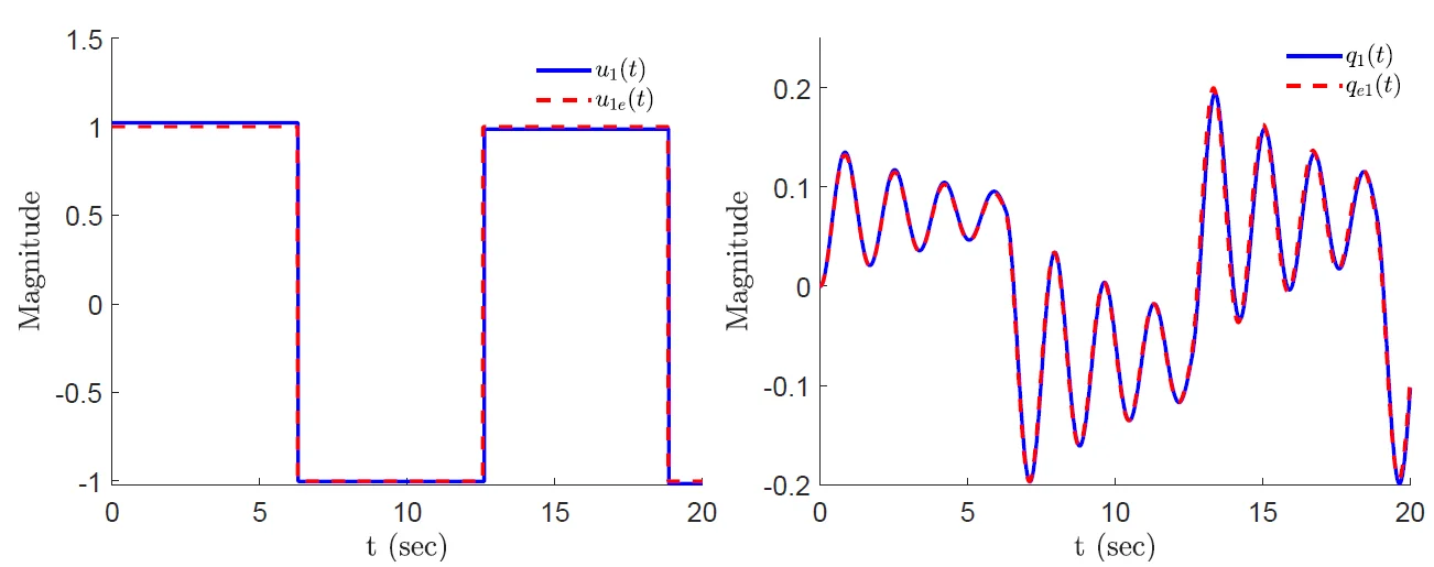
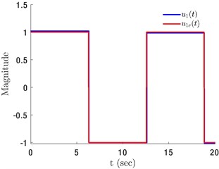
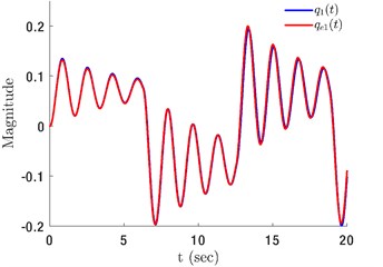
Fig. 1 shows results for the input signal $u_{1e}\left(t\right)$ = $\mathrm{s}\mathrm{g}\mathrm{n}\left(\mathrm{s}\mathrm{i}\mathrm{n}\right(0.5t\left)\right)$. The B-spline parameters considered for this case are $N_c$ = 5 and $k$ = 0, and the homotopy gain parameter $\mathrm{\Gamma }$ = 500. It can clearly be seen from Fig. 1(a) that the identified input $u_1\left(t\right)$ is nearly identical to the actual input $u_{1e}\left(t\right)$. Fig. 1(b) shows the comparison between experimental displacement $q_{1e}\left(t\right)$ and displacement obtained by integrating the mathematical model $q_1\left(t\right)$ with the identified input $u\left(t\right)$. From Fig. 1(b) it is clear that $q_1\left(t\right)$ matches very closely with the experimental data $q_{1e}\left(t\right)$.

Fig. 1a) Actual input u1e(t)=sgn(sin(0.5t)) and identified input u1(t), b) experimental displacement q1e(t), and model displacement q1(t) obtained using u1(t)

a)

b)

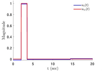
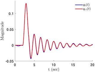
Fig. 2 shows results for the input signal $u_{1e}\left(t\right)=u(t-2)-u(t-3)$. The B-spline parameters considered for this case are $N_c=$6 and $k$ = 0, and the homotopy gain parameter $\mathrm{\Gamma }$ = 150. It can clearly be seen from Fig. 2(a) that the identified input $u_1\left(t\right)$ is nearly identical to the actual input $u_{1e}\left(t\right)$. Fig. 2(b) shows the comparison between experimental displacement $q_{1e}\left(t\right)$ and displacement obtained by integrating the mathematical model $q_1\left(t\right)$ with the identified input $u\left(t\right)$. From Fig. 2(b) it is clear that $q_1\left(t\right)$ matches very closely with the experimental data $q_{1e}\left(t\right)$.

Fig. 2a) Actual input u1e(t) = rect(t), 2≤t≤3 and identified input u1(t), b) experimental displacement q1e(t), and model displacement q1(t) obtained using u1(t)

a)

b)

6. Conclusions

In this work, the input reconstruction problem for non-linear dynamical systems is studied. Through input vector parameterization, the unknown input identification problem is reformulated as a parameter identification problem, which is then solved using the ideas of Homotopy transformation. Homotopy transformation is considered so that the global optimum is achieved. A theoretical analysis of the homotopy transformation is presented in this work, in which it is shown that as long as the high-gain observer synchronizes the experimental and model response, the global optimum of the objective function can be identified. Finally, the accuracy of the proposed methodology is demonstrated via a numerical example in which it is shown that by using the proposed methodology one can effectively reconstruct the unknown inputs.