Abstract
The Huge vibration data are generated continuously by many sensors in daily high-speed rotating machinery operations. Accurate online prediction based on big vibration data streaming can reduce the risks related to failures and avoid service disruptions. This paper presents a hybrid nonlinear autoregressive network with exogenous inputs (NARX) model to forecast the remaining useful life of ball bearings through health index based on big vibration data streaming. This approach is validated by a real data from PRONOSTIA experimentation platform and industrial test rig compared with backpropagation neural network (BP), Elman and general regression neural network (GRNN) prediction model. Root mean square error, mean absolute error and correlation coefficient were used as performance indexes to evaluate the prediction accuracy of these models. The mean absolute error, the root mean square error and the correlation coefficient of hybrid NARX model evaluation index are 2.04, 2.85 and 0.98 respectively. It shows that the model presented in this paper has higher prediction accuracy. It can meet the needs of actual ball bearing remaining useful life prediction and also provide reference in other fields.
1. Introduction
With the development of data acquisition, storage and analysis technology, big data analysis and application have become possible. Streaming data analysis is a kind of big data analysis technology. Streaming data analysis of big data is becoming a hot research topic in recent years [1-6]. The vibration data of ball bearing sensor is a kind of big stream data. For example, in 2012, Italy Ministry of Communications Statistics about 600000 bearings in the country. According to the literature, it is known that the data volume obtained by vibration sensors will be very large [7, 8]. Many scholars have made a lot of useful explorations for predicting the remaining useful life of ball bearings with a large number of vibration data. Guo et al. used recurrent neural network to build health index in order to predict the remaining useful life of ball bearings [9]. Wang et al. built health index via multiple statistical indicators and Mahalanobis distance. Then, an enhanced Kalman filter and EM hybrid algorithm were used to predict the remaining useful life of bearing adaptively [10]. Zhao et al. proposed a hybrid method of time frequency representation and supervised dimensionality reduction in order to predict bearing remaining useful life [11]. Every observation has 25,600 dimensions’ feature. Wu et al. used moving average to reduce the impact of noise in the bearings signal and apply BP to estimate the life percentile and failure times of bearings [12]. Gebraeel et al. used BP to predict bearing failure times [13]. Wang et al. used PCA and improved logistic regression model to predict remaining useful life of rolling bearing [14]. Wang et al. used time domain, frequency domain, time-frequency domain feature as the original features from the bearing vibration signals. Although these health indexes got good results for predicting bearing remaining useful life, there are still some drawbacks which are needed to be solved. For example, Zhao, Wang and Guo’s methods of building health indices are complex and inefficient in the case of big streaming data. Another example is the moving average method is simple and can effectively eliminate the stochastic fluctuation in the prediction, but it makes the predicted value less sensitive to the actual change of the data and the timeliness is bad. It is a great challenge to design an effective remaining useful life scheme of ball bearing based on vibration big data, considering computing resources, calculation time and prediction accuracy rate. One of the challenges is to build an effective health indicator from the massively abundant vibration sensors stream data. The second challenge is the computational accuracy and time of the prediction model.
In order to address the aforementioned shortcomings, this paper presents a health index and grey NARX model in order to predict ball bearing remaining useful life. Based on the health index, a modeling study on the prediction of residual life of ball bearing is carried out. In terms of model research, BP, Elman, NARX and GRNN prediction model were established respectively, and the experimental results were analyzed.
The rest of this paper is organized as follows. In Section 2, a new health index method is put forward for preprocessing original vibration data in order to improve the data quality. Then, the generalized grey neural network prediction framework is used to predict the remaining useful life of ball bearings. The effectiveness of the proposed model is verified by comparative experiments using PRONOSTIA data and industrial bearing data in section three. Finally, conclusions are drawn in the last section.
2. Health index and proposed neural network architecture
This section introduces health index and describes NARX for predicting the remaining useful life of ball bearings.
Firstly, the health index of ball bearings was got by Eq. (1) using the original streaming vibration data:
where represents the maximum value in the data segment, refers to the minimum value in the data segment, and variance is the degree of dispersion of all data in the data segment.
To illustrate the significance of health index, an example is given. Assume two sets {0; 8; 12; 20} and {8; 9; 11; 12}, they have the same average, 10. The following data can be obtained by calculation. The variance of is 69.33. The variance of is 3.33. of is 693.33. of is 6.67. From the result of calculations, it can be learned that the health index reflects the overall size and range of data set. Therefore, the health index can reflect the range and overall size of vibration data of the sample files during the bearing working process.
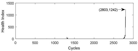
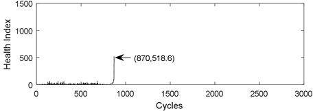
Fig. 1 shows the challenges in predicting the remaining useful life of ball bearings. The curve in Fig. 1(a) shows the health index of life cycle data of PRONOSTIA ball bearing 1-1. The curve in Fig. 1(b) displays the health index of life cycle data of PRONOSTIA ball bearing 1-2. Two different curves were obtained under the same experimental environment and the same type ball bearings. The life span of bearing 1-1 is 2803 cycles, but it is 870 cycles for bearing1-2. The health index of bearing 1-1 is 1242, while the health index of bearing 1-2 is 518.6. On the one hand, it is difficult to find any regular pattern in life span and a threshold. On the other hand, Fig. 1 demonstrates that health index of ball bearing is a non-monotone oscillation sequence.
Secondly, a hybrid method is introduced to predict the remaining useful life of ball bearings based on health index from vibration signals. Neural network with nonlinear mapping characteristics is introduced to help predict data and reduce prediction error. This paper proposed grey NARX model in order to forecast ball bearings remaining useful life.
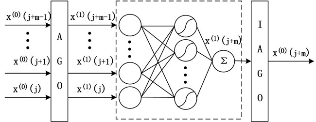
The first step of the proposed model is to preprocess the health index according to accumulated generating operation (AGO) method in grey theory, and get the input data which NARX needs. The second step is to get cumulative prediction based on input data and NARX algorithm. The third step is to get the prediction data of health index through inverse accumulated generating operation (IAGO) method.
The original health index was set to Recorded as . A new series was got by using cumulative sum according to the series :
where and .
Fig. 1Health index from the same type bearing and the same test conditions: a) bearing 1-1, b) bearing 1-2
a)
b)
Applying dynamic neural networks for modeling and predicting data series is the major application of these networks. NARX is a type of recurrent dynamic neural network. NARX is an effective approach to solving nonlinear sequence problems [15].
NARX neural network model can be written as:
where and are the input and target data, respectively. The maximum lags of and are and , respectively. is a nonlinear mapping function. is the output of NARX neural network.
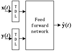
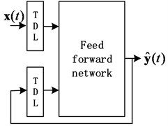
There are two different types of NARX neural networks, open-loop NARX and close-loop NARX. They can be described by Eq. (4) and (5), respectively:
where is the output at time , is the true past values set of the sequence. is the inputs set of the network. The number of output delays is and is the number of input lags. is the past predicting values set of the sequence. The difference between open loop architecture and closed loop architecture is that open loop architecture uses the true past values and closed loop architecture uses predictive past values .
Fig. 2Architecture of NARX: a) open loop architecture, b) close loop architecture
a)
b)
In general, the training time of close loop is much longer than that of open loop and NARX neural network obtained by close loop training is often worse than NARX neural network obtained from open loop training. Therefore, NARX model is trained in open loop architecture and is used in closed loop architecture for multi-step prediction in this paper.
The predicted value of the original sequence is solved by the cumulative predicted value sequence by Eq. (6). This process is called IAGO:
To verify the performance of the proposed model, this paper used grey neural network architecture [16-19]. Fig. 3 describes the generalized grey neural network architecture. is a fragment of the streaming health data. AGO is used to preprocess the original data into approximate monotonic sequence data [19]. The purpose of this transformation is to weaken the random fluctuation in series data. A neural network is represented in the dotted line frame. It can be a static neural network, or a dynamic neural network. For example, BP and GRNN are common static neural networks. For instance, Elman and NARX are common dynamic neural networks. Finally, the predictive value of the original vibration time series can be got by IAGO.
Fig. 3Generalized grey neural network prediction framework
3. Experimental study
The remaining useful life of ball bearings is closely related to the load, temperature and other factors in working environment. In the running process, the real-time monitoring signal of the ball bearing’s vibration and temperature can reflect the current running state. The use of vibration signals to predict remaining useful life of ball bearings is the most widely used and most effective method at present. Considering the non-linear and nonstationary characteristics of the vibration signals of ball bearings, this section uses health index of ball bearings. BP, GRNN and Elman prediction model combined with grey data preprocessing method are applied to evaluating the proposed grey NARX model using the PRONOSTIA accelerated life test data of ball bearings and industrial ball bearing test data.
3.1. Experimental setup
This subsection describes the preparation and related knowledge for vibration stream remaining useful life data prediction of ball bearings.
3.1.1. Datasets description
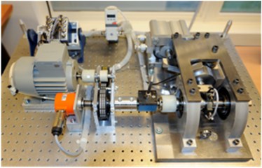
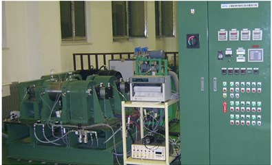
Two experimental data sets of PRONOSTIA and industrial dataset are used to do experiments. These data are obtained from the test rig sensors in Fig. 4.
Fig. 4Ball bearing test rig: a) PRONOSTIA, b) high speed train traction motor bearing test rig
a)
b)
Firstly, PRONOSTIA dataset has been used in many remaining useful life prognostic studies [7, 9, 11, 15]. There are 17 run-to-failure datasets in order to study the prediction of bearing remaining useful life. Vibration and temperature signals have been saved in ASCII files respectively. Since vibration data are studied in this paper, only vibration data are described as follows. The vibration signal consists of a horizontal vibration signal and a vertical vibration signal. The sampling frequency is 25.6 kHz. 2560 samples are recorded every 10 seconds. Each record is stored in an ASCII file. For each ASCII file, the data obtained by the vibration sensor includes the horizontal direction of vibration data and the vertical direction of vibration data. In addition, the corresponding vibration time is also stored in the ASCII file.
Secondly, the industrial ball bearing test of high-speed train is conducted on NTN bearing test rig. The bearing type of high-speed train is 6311 deep groove ball bearing. Acceleration sensor was used to collect vibration signals of ball bearings in order to monitor bearing health condition. The minimum recording period of the test bed is 10 seconds. The cumulative operation time of two experimental bearings is approximately 3000 and 700 hours. All samples are stored in two database files.
3.1.2. Data preprocessing
PRONOSTIA vertical vibration data is extracted from each sample ASCII file. For vertical vibration data of each sample file, Eq. (1) is used to calculate the time series health index. And then the health index vector is then obtained. Fig. 5 describes the whole life cycle health index of the bearing 1-1. As can be seen from Fig. 5, the health index after AGO is smoother and larger than the original data and moving average health index.
Fig. 6 describes the part health index of the bearing1-1 from 1250 to 1350 time unit. From Fig. 5 and 6, it can be seen that the health index processed by MA method is not good at eliminating random fluctuations compared with AGO method. Compared with MA method, AGO method has a large difference value in health index at the same time interval. Since AGO method is more sensitive to data change and has good timeliness, the health index data processed by AGO is used to predict the remaining life of ball bearings.
Fig. 5Health index of the bearing 1-1: a) health index, b) moving average (q= 10) health index, c) accumulated generating operation health index

a)

b)

c)
Fig. 6Part health index of the bearing 1-1: a) health index, b) moving average (q= 10) health index, c) accumulated generating operation health index

a)

b)

c)
3.1.3. Time window processing
Before using the model to predict the nonlinear time series, it is necessary to reconstitute the data format. Suppose the time series is . After reconstructing the data with window size , we get the multi-dimensional feature matrix and the prediction vector . and can be expressed in Eq. (7) and Eq. (8) respectively:
For the feature vector , the expression form is :
The expression form of is .
Fig. 7 describes the reconstruction process of the feature vector and the prediction vector when the window width is 4. The training set for model training is .
Fig. 7Reconstruction of health index time series data

3.1.4. Performance metrics
The performance metrics are mean absolute error (MAE), root mean square error (RMSE) and Pearson’s correlation coefficient ().
MAE is a measure of difference between two variables. It is given by the following equation:
where refers to the sample size, is the predictive value indexed with , is the observed value indexed with . MAE output is non-negative value. The best value is 0.
RMSE is a measure of the differences between model predictive values and the actually observed values. RMSE is given by:
where is the sample size, is the predictive value indexed with , is the observed value indexed with t. A smaller RMSE value implies a smaller error variation between predicted values and observed values. RMSE reflects the degree which the predicted values deviate from the observed values.
is a measure of the linear correlation between two variables. The equation for is:
where refers to the sample size, and are the single sample indexed with , is the mean of data set , is the mean of data set . The value range is between –1 and 1, where –1 is total negative linear correlation, 0 is no linear correlation, and 1 is total positive linear correlation.
3.1.5. Compared approaches
Four methods are used in this paper, which are BP neural network, GRNN, Elman and NARX. BP and GRNN are static neural network. Elman and NARX neural network are dynamic neural networks. Static neural networks are characterized by no feedback, no memory, and the output depends only on the current input. The output of dynamic neural networks with feedback depends not only on current and previous inputs, but also on previous outputs.
BP was put forward by the scientific research group headed by Rumelhart and McCelland in 1986 [20]. BP neural network is a multilayer feed-forward network trained by the error back-propagation algorithm. It is one of the most widely used neural network models. The basic idea of BP is that the learning process consists of two processes, namely, the signals of feedforward and the back-propagation of errors. When forward propagation, the input samples are sent from the input layer, and processed by the hidden layers, and then transmitted to the output layer. If the actual output of the output layer is not consistent with the expected output, it will go back to the error back-propagation stage. In back-propagation, the output is retransmitted to the input layer by the hidden layer in some form, and the error is apportioned to all the units of each layer, thus the error signal of each layer is obtained. The error signal is the basis of correcting the weight of each unit. BP neural network is composed of input layer, hidden layer and output layer. Considering the regression prediction problem here, the transfer function used in BP network is tansig function.
GRNN was proposed by Specht in 1991 [21]. GRNN is a one-pass learning algorithm. Its network structure is highly parallel. GRNN can be used for nonlinear prediction. GRNN is a solution for online dynamical systems. It is a kind of radial basis neural network [22]. The network structure of GRNN is composed of four layers, namely, input layer, pattern layer, summation layer and output layer. Its network input is , and the output is . GRNN model can be expressed as Eq. (12):
where is the prediction value of input . is the activation weight for the pattern layer neuron at . is the Gaussian kernel as formulated .
In 1990, Elman proposed the Elman network, which is a kind of recurrent neural network [23]. Elman neural network is used in many fields, such as cognitive science, economics and others. Elman network structure consist of four layers: input layer, hidden layer, context layer and output layer. The context layer can provide a short memory. Elman networks are used for predicting time series. Elman neural network model can be expressed as Eq. (13):
where is output vector. is the transfer function of output neurons. is the transfer function of middle layer neurons. is hidden layer vector. is a feedback state vector. is input vector. is the connection weight of the middle layer to the output layer. is the connection weight of the input layer to the middle layer. is the connection weight of the context layer to the middle layer.
NARX is a dynamic neural network. NARX can learn to predict time series given past values of the same time series, the feedback input, and the exogenous time series. It can be applied for predicting nonlinear sequence data. It can be used as a recurrent dynamic neural network to predict the next value of the input data.
3.2. Experiment and analysis
This subsection describes experimental process and analyses experimental results.
3.2.1. Experimental process
Our goal is to provide multi-step ahead prediction of ball bearings health index. One step ahead is to predict the next data using historical data in a fixed window. For multi-step ahead predicting, the first step is predicted by applying one step ahead predicting. Subsequently, the predicted value is included as the latest component of input series to predict the next step using the one step ahead training method. This procedure is repeated for the continuous predicting. The following content briefly describes the basic steps in experimental research. Firstly, raw data set is from the vertical vibration streaming data of PRONOSTIA ball bearings and industrial ball bearing test data. Secondly, health index feature is extracted by Eq. (1). Thirdly, the data format required by the grey neural network framework is reconstructed by using the time window processing technique. Fourthly, the learning set 1 includes AGO health indexes from Bearing 1-1, Bearing 1-2, Bearing 1-3, Bearing 1-4, Bearing 2-1, Bearing 2-2, Bearing 2-3 and Bearing 2-4. The learning set 2 includes AGO health indexes from bearing 6311-1. The test set 1 consists of 8 AGO health indexes: Bearing 1-5, Bearing 1-6, Bearing 1-7, Bearing 2-5, Bearing 2-6 and Bearing 2-7. The test set 2 is AGO health index of bearing 6311-2. The learning set is divided into training set, validation set and test set, and the corresponding allocation ratio is 75 %, 15 %, 15 %. Fifthly, BP, GRNN, Elman and NARX learn on the learning set respectively in order to predict the health index of ball bearings remaining useful life. Finally, the training model is used to predict the test set. MAE, RMSE, and test running time are used to evaluate the performance of the four neural networks on the test set.
3.2.2. Performance comparison
The experimental results are divided into two parts. The first part is the life prediction result of ball bearing life cycle. The second part is the prediction result of the later period life of ball bearings. A comparison of the predicted and real values of the four algorithms in the two bearing test sets is shown in Fig. 8 and Fig. 9. The experimental performance results of two test sets are summarized in Table 1, Table 2, Table 3 and Table 4.
From Fig. 8, it can be seen that BP and GRNN methods are getting smaller and smaller with the increasing number of data obtained. This is not good for predicting the remaining useful life of ball bearings with relatively short life. With the increasing number of data acquired by sensors, Elman and NARX method prediction error is relatively stable. This is beneficial for predicting the residual service life of the ball bearings. From the results in Fig. 9, it can be seen that the prediction error of four methods on test set 2 is BP, GRNN, Elman and NARX in descending order.
Table 1 shows the performance of four different models. Results are expressed as mean ± SD. After calculation, the value of MAE, RMSE and indexes of BP are 49.71±15.84, 53.77±12.87 and 1.00±0.01 respectively. The test running time required for BP on the test set 1 is 0.01±0.00 seconds. The value of MAE, RMSE and indexes of GRNN is 40.51±10.55,44.89±8.43 and 0.99±0.01 respectively. The test running time required for GRNN on the test set is 0.27±0.17 seconds. The value of MAE, RMSE and indexes of Elman is 6.84±1.38, 7.54±1.46 and 1.00±0.00 respectively. The average time required for Elman on the test set is 0.01±0.00 seconds. And the value of MAE, RMSE and R indexes of NARX is 1.60±1.41 2.94±3.04 and 0.99±0.02 respectively. The test time required for NARX on the test set is 0.03±0.01 seconds. By comparison, the performance index of NARX were significantly higher than that of BP, Elman and GRNN. GRNN test runs for the longest time in four models. The other three models have a similar test run time. As it can be observed, compared with other methods, NARX method is more suitable for continuous prediction than the other methods using PRONOSTIA data.
Fig. 8Comparison: a) bearing 1-5, b) bearing1-6, c) bearing 1-7, d) bearing 2-5, e) bearing 2-6, f) bearing 2-7

a)

b)

c)

d)

e)

f)
Fig. 9Comparison of 4 algorithms on bearing 6311 life cycles

a)

b)

c)

d)

e)

f)
Considering the late prediction of the remaining useful life of ball bearings is more important, the last one hundred health indexes are selected for comparison. It can be calculated from Table 2 that the values of MAE, RMSE and of BP are 59.14±36.36,59.29±36.28 and 1.00±0.01 respectively. The test time required for BP on the test set 1 is 0.01±0.00seconds. The values of MAE, RMSE and of GRNN are 22.92±15.58, 23.43±16.27 and 1.00±0.01 respectively. The test time required for GRNN on the test set 1 is 0.03±0.02 seconds. The values of MAE, RMSE and R of Elman are 9.78±3.27, 9.99±3.18 and 1.00±0.01 respectively. The test time required for Elman on the test set 1 is 0.01±0.00 seconds. And the values of MAE, RMSE and of NARX are 2.04±2.16,2.85±3.53 and 0.98±0.03 respectively. The test time required for NARX on the test set 1 is 0.01±0.00 seconds. After analysis, BP is still the worst of the four hybrid models. However, the average performance of the last part of the GRNN model is lower than that of the total data. The average value of MAE and RMSE index of Elman method is lower than that of GRNN, but higher than that of NARX. The average values of MAE, RMSE and of NARX are the lowest among the four methods. The average performance of the last part of the NARX method is quite similar to the average performance of the whole life cycle data. According to the calculation results of Tables 1 and 2, grey NARX predict model has a higher prediction accuracy for predicting the remaining useful life of PRONOSTIA ball bearings.
From Table 3, it can be seen that BP has the largest MAE and RMSE on the test set 2, while the MAE and RMSE of NARX are the smallest. The four algorithms are almost completely positively correlated. The test run time of GRNN is the most, while the test run time of the other models is approximately equal. As can be seen from Table 4, the results of prediction performance of bearing 6311 last 100 health indexes and prediction performance of bearing 6311 all health indexes were similar. Because of the test rig conditions, time and financial constraints, only two bearings were used for the experiment. If the number of bearings increases, the prediction error of industrial bearings will be further reduced in real scenarios. As can be seen from table 1-4, grey NARX is the most suitable model for continuous prediction the remaining useful life of ball bearings than other three models.
Table 1Prediction performance of PRONOSTIA all health indexes
Algorithm | Bearing No | MAE | RMSE | Test time (s) | |
BP | Bearing 1_5 | 38.039 | 43.801 | 1.000 | 0.010 |
Bearing 1_6 | 43.346 | 51.076 | 1.000 | 0.008 | |
Bearing 1_7 | 42.629 | 46.914 | 1.000 | 0.007 | |
Bearing 2_5 | 34.785 | 41.203 | 1.000 | 0.008 | |
Bearing 2_6 | 68.565 | 68.587 | 1.000 | 0.008 | |
Bearing 2_7 | 70.918 | 71.022 | 0.987 | 0.007 | |
– | 49.71±15.84 | 53.77±12.87 | 1.00±0.01 | 0.01±0.00 | |
GRNN | Bearing 1_5 | 27.889 | 35.421 | 0.990 | 0.520 |
Bearing 1_6 | 34.777 | 40.549 | 0.992 | 0.396 | |
Bearing 1_7 | 33.201 | 38.861 | 0.981 | 0.255 | |
Bearing 2_5 | 43.559 | 46.867 | 0.981 | 0.289 | |
Bearing 2_6 | 47.087 | 49.004 | 0.999 | 0.139 | |
Bearing 2_7 | 56.574 | 58.654 | 0.984 | 0.037 | |
– | 40.51±10.55 | 44.89±8.43 | 0.99±0.01 | 0.27±0.17 | |
ELMAN | Bearing 1_5 | 8.742 | 9.526 | 1.000 | 0.019 |
Bearing 1_6 | 7.281 | 8.255 | 1.000 | 0.012 | |
Bearing 1_7 | 5.056 | 5.972 | 1.000 | 0.009 | |
Bearing 2_5 | 6.115 | 6.822 | 1.000 | 0.008 | |
Bearing 2_6 | 5.935 | 6.077 | 1.000 | 0.009 | |
Bearing 2_7 | 7.913 | 8.602 | 0.989 | 0.008 | |
– | 6.84±1.38 | 7.54±1.46 | 1.00±0.00 | 0.01±0.00 | |
NARX | Bearing 1_5 | 1.298 | 1.783 | 1.000 | 0.040 |
Bearing 1_6 | 3.065 | 6.409 | 1.000 | 0.038 | |
Bearing 1_7 | 0.494 | 0.668 | 1.000 | 0.028 | |
Bearing 2_5 | 0.556 | 0.756 | 1.000 | 0.035 | |
Bearing 2_6 | 0.547 | 0.785 | 0.999 | 0.018 | |
Bearing 2_7 | 3.659 | 7.227 | 0.960 | 0.012 | |
– | 1.60±1.41 | 2.94±3.04 | 0.99±0.02 | 0.03±0.01 |
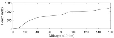
After calculating the health index of the bearing during the entire service process, the relationship between the health index of the bearing vibration data and the running mileage in the bearing life cycle can be obtained, as shown in Fig. 10(a). After getting the relationship between the mileage and the health index, the remainder life of rolling bearings can be obtained by using the design life subtracted from the mileage corresponding to the health index, as shown in Fig. 10(b).
Table 2Prediction performance of PRONOSTIA last 100 health indexes
Algorithm | Bearing No | MAE | RMSE | Test time (s) | |
BP | Bearing 1_5 | 71.569 | 71.595 | 1.000 | 0.009 |
Bearing 1_6 | 110.623 | 110.732 | 0.995 | 0.008 | |
Bearing 1_7 | 28.606 | 29.058 | 1.000 | 0.007 | |
Bearing 2_5 | 7.274 | 7.416 | 1.000 | 0.007 | |
Bearing 2_6 | 66.013 | 66.013 | 1.000 | 0.008 | |
Bearing 2_7 | 70.733 | 70.905 | 0.979 | 0.007 | |
– | 59.14±36.36 | 59.29±36.28 | 1.00±0.01 | 0.01±0.00 | |
GRNN | Bearing 1_5 | 18.185 | 18.196 | 1.000 | 0.083 |
Bearing 1_6 | 12.555 | 12.740 | 0.996 | 0.026 | |
Bearing 1_7 | 3.359 | 3.683 | 0.999 | 0.025 | |
Bearing 2_5 | 26.020 | 26.154 | 1.000 | 0.025 | |
Bearing 2_6 | 28.832 | 28.889 | 1.000 | 0.026 | |
Bearing 2_7 | 48.546 | 50.910 | 0.975 | 0.024 | |
– | 22.92±15.58 | 23.43±16.27 | 1.00±0.01 | 0.03±0.02 | |
ELMAN | Bearing 1_5 | 12.944 | 12.945 | 1.000 | 0.011 |
Bearing 1_6 | 12.201 | 12.312 | 0.995 | 0.008 | |
Bearing 1_7 | 11.006 | 11.009 | 1.000 | 0.007 | |
Bearing 2_5 | 10.582 | 10.583 | 1.000 | 0.008 | |
Bearing 2_6 | 4.155 | 4.159 | 1.000 | 0.008 | |
Bearing 2_7 | 7.821 | 8.951 | 0.981 | 0.008 | |
– | 9.78±3.27 | 9.99±3.18 | 1.00±0.01 | 0.01±0.00 | |
NARX | Bearing 1_5 | 1.080 | 1.160 | 0.998 | 0.011 |
Bearing 1_6 | 3.289 | 4.138 | 0.963 | 0.012 | |
Bearing 1_7 | 1.198 | 1.458 | 0.999 | 0.014 | |
Bearing 2_5 | 0.735 | 0.774 | 0.999 | 0.010 | |
Bearing 2_6 | 0.063 | 0.076 | 1.000 | 0.010 | |
Bearing 2_7 | 5.859 | 9.476 | 0.937 | 0.010 | |
– | 2.04±2.16 | 2.85±3.53 | 0.98±0.03 | 0.01±0.00 |
Table 3Prediction performance of bearing 6311-2 all health indexes
Algorithm | MAE | RMSE | Test run time (s) | |
BP | 222.431 | 240.475 | 1.000 | 0.050 |
GRNN | 82.048 | 122.780 | 0.955 | 0.085 |
ELMAN | 32.367 | 34.777 | 1.000 | 0.017 |
NARX | 12.911 | 14.375 | 1.000 | 0.016 |
Table 4Prediction performance of bearing 6311-2 last 100 health indexes
Algorithm | MAE | RMSE | Test run time (s) | |
BP | 124.579 | 124.884 | 0.995 | 0.022 |
GRNN | 40.990 | 49.558 | 0.984 | 0.015 |
ELMAN | 19.163 | 19.745 | 0.992 | 0.013 |
NARX | 12.276 | 13.248 | 0.970 | 0.009 |
Fig. 10Relationship between mileage, health index and remaining useful life (RUL)
a)

b)
4. Conclusions
Remaining useful life prediction accuracy highly relies on the performance of health index and predict model. In this paper, BP, GRNN, Elman and NARX neural network model were used to forecast the remaining useful life from the vibration acceleration data of the ball bearing. The results show that the precision of grey NARX neural network model is higher than BP, GRNN and Elman. The predict value of grey NARX neural network model is closer to the actual data, especially when the noise is relatively large. NARX neural network model has shorter prediction time compared with GRNN method. On the other hand, the research on the feature of ball bearing vibration acceleration, not only provides a feasible and effective method for establishing bearing remaining useful life index, also can establish remaining useful life prediction model of ball bearings provide some references. At the same time, the selection of prediction feature is not limited to the vibration acceleration. It can also be used for other features such as temperature. Grey NARX model and health index can be used to realize the remaining useful life prediction of the related components in future.
References
-
Nair L. R., Shetty S. D., Shetty S. D. Applying spark based machine learning model on streaming big data for health status prediction. Computers and Electrical Engineering, Vol. 65, 2017, p. 393-399.
-
Han D., Li S., Wei F., et al. Two birds with one stone: classifying positive and unlabeled examples on uncertain data streams. Neurocomputing, Vol. 277, 2017, p. 149-160.
-
Fernández Rodríguez J.-Y., Álvarez García J.-A., Fisteus J. A., et al. Benchmarking real-time vehicle data streaming models for a smart city. Information Systems, Vol. 72, 2017, p. 62-76.
-
Morales G. D. F., Bifet A. SAMOA: scalable advanced massive online analysis. Journal of Machine Learning Research, Vol. 16, 2015, p. 149-153.
-
Parker B. S., Khan L., Bifet A. Incremental ensemble classifier addressing non-stationary fast data streams. IEEE International Conference on Data Mining Workshops, 2014, p. 716-723.
-
Zeng X. Q., Li G. Z. Incremental partial least squares analysis of big streaming data. Pattern Recognition, Vol. 47, Issue 11, 2014, p. 3726-3735.
-
Fumeo E., Oneto L., Anguita D. Condition based maintenance in railway transportation systems based on big data streaming analysis. Procedia Computer Science, Vol. 53, Issue 1, 2015, p. 437-446.
-
Schoen R. R., Habetler T. G., Kamran F., et al. Motor bearing damage detection using stator current monitoring. IEEE Transactions on Industry Applications, Vol. 31, Issue 6, 1994, p. 1274-1279.
-
Guo L., Li N., Jia F., et al. A recurrent neural network based health indicator for remaining useful life prediction of bearings. Neurocomputing, Vol. 240, 2017, p. 98-109.
-
Wang Y., Peng Y., Zi Y., et al. A two-stage data-driven-based prognostic approach for bearing degradation problem. IEEE Transactions on Industrial Informatics, Vol. 12, Issue 3, 2016, p. 924-932.
-
Zhao M., Tang B., Tan Q. Bearing remaining useful life estimation based on time-frequency representation and supervised dimensionality reduction. Measurement, Vol. 86, 2016, p. 41-55.
-
Wu S., Gebraeel N., Lawley M. A., et al. System for condition-based optimal predictive maintenance policy. IEEE Transactions on Systems, Man, and Cybernetics, Vol. 37, 2007, p. 226-236.
-
Gebraeel N., Lawley M., Liu R., et al. Residual life predictions from vibration-based degradation signals: a neural network approach. IEEE Transactions on Industrial Electronics, Vol. 51, Issue 3, 2004, p. 694-700.
-
Wang F., Wang B., Dun B., et al. Remaining life prediction of rolling bearing based on PCA and improved logistic regression model. Journal of Vibroengineering, Vol. 18, Issue 8, 2016, p. 5192-5203.
-
Rai A., Upadhyay S. H. The use of MD-CUMSUM and NARX neural network for anticipating the remaining useful life of bearings. Measurement, Vol. 111, 2017, p. 397-410.
-
Zeng X. Y., Shu L., Huang G. M., et al. Triangular fuzzy series forecasting based on grey model and neural network. Applied Mathematical Modelling, Vol. 40, Issue 3, 2016, p. 1717-1727.
-
Lei Y., Guo M., Hu D. D., et al. Short-term prediction of UT1-UTC by combination of the grey model and neural networks. Advances in Space Research, Vol. 59, Issue 2, 2017, p. 524-531.
-
Liu X., Moreno B., Garcia A. S. A grey neural network and input-output combined forecasting model. Primary energy consumption forecasts in Spanish economic sectors. Energy, Vol. 115, 2016, p. 1042-1054.
-
Abdulshahed A. M., Longstaff A. P., Fletcher S., et al. Thermal error modelling of a gantry-type 5-axis machine tool using a grey neural network model. Journal of Manufacturing Systems, Vol. 41, 2016, p. 130-142.
-
Rumelhart D. E., Hinton G. E., Williams R. J. Learning representations by back-propagating errors. Nature, Vol. 323, Issue 6088, 1986, p. 533-536.
-
Specht D. F. A general regression neural network. IEEE Transactions on Neural Networks, Vol. 2, Issue 6, 1991, p. 568-576.
-
Tse P. W., Atherton D. P. Prediction of machine deterioration using vibration based fault trends and recurrent neural networks. Journal of Vibration and Acoustics, Vol. 121, Issue 3, 1999, p. 355-362.
-
Elman J. L. Finding structure in time. Cognitive Science, Vol. 14, Issue 2, 1990, p. 179-211.
Cited by
About this article
This work was partially supported by Comprehensive standardization and new mode application project of Intelligent Manufacturing in Ministry of industry and information technology of People's Republic of China No. 2017ZNZZ01-06, the Science and Technology Research and Development Major/Key Program of China Railway Corporation No. 2016J007-B, National Natural Science Foundation of China No.51577007, and Beijing Natural Science Foundation (3162023). Finally, the authors are grateful to the anonymous reviewers for their helpful comments and constructive suggestions.
Qiming Niu put forward the formula of health index. Qingbin Tong discussed the possibility of structure. Junci Cao and Yihuang Zhang did experiments. Feng Liu put forward constructive suggestions.
