An improved variational mode decomposition method and its application in diesel engine fault diagnosis

1. Introduction

The engine is a complex mechanical device, with the characteristics of multi-source, multi moving parts, complex work. The engine has both rotational and reciprocating motion. Vibration signals are fully used in fault diagnosis because of their convenience [1, 2]. The vibration signal of engine is composed of multi-component complex signals, and its amplitude varies with time. For the complex multi-component signal, it is usually necessary to decompose it into a number of single-component AM-FM signals, and each component is analyzed to extract amplitude and frequency information.

Huang et al proposed the Empirical Mode Decomposition (EMD) [3, 4]. EMD has been widely used in mechanical fault diagnosis since it was proposed [5, 6]. EMD is fundamentally divorced from the Fourier transform. EMD analyzes the signal from itself and it is completely adaptive and unsupervised. But there are some problems for EMD, such as endpoint effect and modal aliasing [7].

Wu [8] proposed Ensemble Empirical Mode Decomposition (EEMD). Different white noises are added to the original signal for EMD, and multiple decomposition results are averaged to obtain the final Intrinsic Mode Function (IMF). The high frequency modulation information in the signal can be separated very well, and the modal aliasing of EMD is well suppressed [9]. Torres [10] proposed a Complete Ensemble Empirical Mode Decomposition with Adaptive Noise (CEEMDAN). The method reduces the reconstruction error caused by white noise while suppressing the aliasing of modes. However, the two methods share a common flaw. Their computation is very large and a lot of pseudo components will appear in the decomposition process.

Smith proposed the Local Mean Decomposition (LMD) [11]. LMD considers that a complex single-component signal is the product of its own envelope signal and an FM signal, which is called Product Function (PF). A complex signal is decomposed into several PF components with the physical meaning of instantaneous frequency. LMD avoids the problems of over envelope, incomplete envelope and negative frequency caused by Hilbert transform in EMD. However, LMD also has some problems such as frequency aliasing and endpoint effect [12]. Mark G Frei [13] proposed the Intrinsic Time-scale Decomposition (ITD). Any complex signal can be decomposed into several independent Proper Rotation (PR) components, and its instantaneous frequency is of physical significance. However, baseline definition in LMD is based on the linear transformation of the signal itself. So, from the second components, the components are different from the usual definition of IMF, and an apparent signal distortion occurs. Then the instantaneous amplitude and instantaneous frequency are distorted greatly [12].

In recent years, Konstantin Dragomiretskiy [14] proposed a new variable adaptive decomposition method, Variational Mode Decomposition (VMD). The method is essentially composed of a plurality of adaptive Wiener filter and has good noise robustness. Compared with EMD, VMD has strong mathematical theory basis. At the same time, VMD rejects the method of recursive screening stripping. So VMD can effectively alleviate or avoid a series of problems which appear in EMD, and has high operation efficiency of decomposition [15]. VMD has been fully utilized in the field of engineering [16-19].

However, it is a problem that how to determine the number of decomposition layers and the penalty factor, because human factors will affect the decomposition results. Genetic algorithm is a global optimization random probability search algorithm that simulates the inheritance and variation of chromosomes in a population based on natural selection and natural genetic mechanism in the biological world. Genetic algorithm is often used in parameter optimization, and has fast convergence speed and wide adaptability. Genetic algorithms mainly include 3 genetic operators: selection, crossover and mutation. The cross probability and mutation probability will directly affect the optimization results. In the traditional genetic algorithm, the probability of cross and mutation are fixed, and the genetic algorithm is easy to fall into the local optimal [20]. M. Srinvas [21] proposed an adaptive genetic algorithm, which could adaptively adjust the cross probability and mutation probability in the genetic algorithm. As a result, the convergence rate is improved, but there is an evolutionary stagnation at the early stage of evolution. In order to solve the problem, an improved adaptive genetic algorithm (IAGA) was proposed to optimize the modal number $K$ and penalty factor $\alpha$ of VMD in this paper. According to the law of hormone regulation, the cross probability and mutation probability in evolution were improved. Compared with the traditional adaptive genetic algorithm, the convergence speed is faster and the local optimum is avoided. Based on the proposed method, the vibration signal of diesel engine crankshaft was analyzed. The result shows that the proposed method can quickly converge to the global optimal value and have high stability.

2. Variational mode decomposition

The VMD algorithm defines the intrinsic mode function as a non-stationary AM-FM signal. The intrinsic mode is considered as follows:

where the phase ${\phi }_k\left(t\right)$ shall satisfy the following condition: ${\phi }_k{\left(t\right)}^{\mathrm{\text{'}}}\ge$ 0; the envelope line $A_k\left(t\right)$ should satisfy the following condition: $A_k\left(t\right)\ge$ 0; the instantaneous frequency ${\omega }_k\left(t\right)$ should satisfy the following condition: ${\omega }_k\left(t\right)={\phi }_k{\left(t\right)}^{\mathrm{\text{'}}}$. $A_k\left(t\right)$ and ${\omega }_k\left(t\right)$ change slowly, and ${\phi }_k\left(t\right)$ changes more rapidly.

The Hilbert transform is performed for each modal function $u_k\left(t\right)$, and exponential correction is applied to obtain $K$ modal functions. Then the frequency spectrum of the modal function is corrected to the estimated central frequency, and the bandwidth of the modal component is calculated by using Gauss smoothing. The variational constraint problem can be defined as follows:

where $u_k$ is the modal component, ${\omega }_k$ is the central frequency for the modal component, $\delta \left(t\right)$ is the unit pulse function, and * is the convolution symbol.

In the VMD algorithm, the secondary penalty factor and the Lagrangian multiplication operator are used. Then, the alternating direction method is introduced. $u_k^{n+1}$, ${\omega }_k^{n+1}$, and ${\lambda }^{n+1}$ are constantly updated, so that the optimal solution of the variational constraint problem can be solved. The expression for the modal component $u_k^{n+1}$ is:

where $\alpha$ is the penalty factor, and $\lambda$ is the Lagrange multiplier.

The expression for the modal component $u_k^{n+1}$ in frequency domain is:

where ${\omega }_k$ is the center of the modal component power spectrum. The Wiener filter is introduced, which makes the VMD algorithm have better noise robustness.

Similarly, the expression for the central frequency ${{\omega }_k}^{n+1}$ is:

The stopping condition of the iteration is:

The VMD algorithm is a linear transformation, so the signal can be reconstructed. The reconstructed signal can be represented as:

where ${\widehat{u}}_k$ is the final modal component, after the iteration is stopped.

3. Improved adaptive genetic algorithm

Genetic algorithm is a global optimization random probability search algorithm that simulates the inheritance and variation of chromosomes in a population based on natural selection and natural genetic mechanism in the biological world. Genetic algorithms mainly include 3 genetic operators: selection, crossover and mutation. The cross probability and mutation probability will directly affect the optimization results. When the fitness of individuals is lower than the average fitness, the probability of crossover and mutation should be improved. If the fitness of individuals is higher than the average fitness, the probability of crossover and mutation should be reduced. The cross probability and mutation probability in the traditional genetic algorithm are fixed. As a result, the genetic algorithm is easy to fall into the local optimal.

M. Srinvas [21] proposed an adaptive genetic algorithm to adaptively adjust the cross probability and mutation probability in the genetic algorithm:

where $P_c$ is the cross probability; $P_m$ is the mutation probability; $f\mathrm{\text{'}}$ is the larger fitness of the two individuals involved in the cross; $f$ is the individual’s fitness value for a mutation operation; $f_{max}$ is the maximum fitness value in the population; $f_{min}$ is the smallest fitness value in the population; $k_1$, $k_2$, $k_3$ and $k_4$ are constants in the range of (0,1). According to Eqs. (12) and (13), the convergence rate of the adaptive genetic algorithm is improved. However, there is an evolutionary stagnation at the early stage of evolution for the adaptive genetic algorithm.

In order to solve the above problems, according to the law of hormone regulation, the following improvements are made to optimize the cross probability and mutation probability in evolution:

where $P_c^0$ is the initial cross probability; $P_m^0$ is the initial mutation probability; $\gamma$, $\beta$, $k_c$ and $k_m$ are coefficient factors. Through the above improvement, the individual is more diverse, and the problems of premature convergence and slow evolution are effectively solved.

4. Proposed method

According to the VMD algorithm introduced in the chapter 2, VMD needs a given decomposition mode number $K$ during the decomposition process, and the value of $K$ has a great influence on the decomposition results. In addition, the penalty factor $\alpha$ in the algorithm also has a great influence on the decomposition results. If the modal number $K$ and the penalty factor $\alpha$ are set artificially, the decomposition results will be subject to subjective influence. It is a prerequisite for VMD that how to set these two parameters.

The IAGA is a global optimization random probability search algorithm, which avoids the problem of premature convergence and slow evolution. Therefore, the IAGA is used to optimize the modal number $K$ and penalty factor $\alpha$ of VMD in this paper, and the optimal input parameters are obtained.

In the process of optimization, IAGA needs to define a fitness function. The permutation entropy is a new method of mutation detection, which mainly aims at the spatial characteristics of time series [22, 23]. The permutation entropy is very simple in theory and has good noise robustness. Besides, the permutation entropy also has a high resolution, and the output results are very intuitive. The permutation entropy reflects the random degree of the signal. In other words, the smaller the permutation entropy, the more regular the time series is; the larger the entropy, the more random the time series is. In phase space, a set of time series $X\left(i\right)$ is reconstructed to get a set of symbol sequence, and the probability of each symbol sequence appears as $P_1$, $P_2$, …,$\mathrm{}{P}_k$. Then the permutation entropy of the time series $X\left(i\right)$ can be defined as:

when the crankshaft of a diesel engine fails, it is often accompanied by the violent vibration and abnormal noise of the body. If the fault features are obvious, the signal has periodic fluctuation and the permutation entropy is relatively small. If there is a lot of noise in the signal, the randomness of the signal is large, and the permutation entropy is relatively large. Therefore, the fitness function of IAGA is the permutation entropy of the components obtained by VMD. When the signal is decomposed by VMD, the minimum permutation entropy is called the local minimum permutation entropy value, and the corresponding component is the local optimal component. Then the local minimal permutation entropy is used as the fitness value of the whole evolutionary process to search the optimal combination of parameters. The signal is decomposed by the optimized VMD, and the component with the minimum permutation entropy is selected as the fault component to extract the feature.

5. Experimental results

5.1. Simulation

The simulation signal is set up to verify the decomposition effect of the VMD optimized by IAGA. The engine structure is complex, and the vibration excitation source is multitudinous. Besides, the engine often operates in transient conditions, and the source vibration signal is modulated by a plurality of components. Therefore, the simulation signals of the engine must satisfy the requirements of multi- component, non-stationary and AM-AF signals. In this paper, Gauss noise is added to the simulation signal, which is more in line with the actual vibration signal characteristics of the diesel engine. The simulation signal is composed of the following:

13

$a={e^{-8(t-0.5)}}^2,$

14

$s_1=a\mathrm{s}\mathrm{i}\mathrm{n}(2\pi \left(100t+\mathrm{c}\mathrm{o}\mathrm{s}\left(5\pi t\right)\right),$

15

$s_2=a\mathrm{s}\mathrm{i}\mathrm{n}\left(2\pi \left(150t+50t^2\right)\right),$

16

$s_3=a\mathrm{s}\mathrm{i}\mathrm{n}\left(2\pi \left(250t+80t^3\right)\right),$

17

$s=s_1+s_2+s_3+0.1\mathrm{r}\mathrm{a}\mathrm{n}\mathrm{d}\mathrm{n}\left(\mathrm{s}\mathrm{i}\mathrm{z}\mathrm{e}\left(s_1\right)\right).$

The signal sampling frequency is 1500 Hz, and the sampling number is 1024. The time domain waveform of the simulation signal components are shown in Fig. 2. As shown in Fig. 2, the simulation signal consists of three non-stationary AM-FM signals. The time-domain and frequency-domain waveforms of the noisy simulation signals are shown in Fig. 3. The composition and variation of the signal are not clear from Fig. 3. We don't know what the signal contains.

Fig. 1Detailed experimental scheme

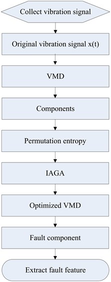
Fig. 2The source components of simulation signal

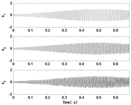
Fig. 3The simulation signal and its spectrum

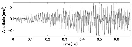
a)

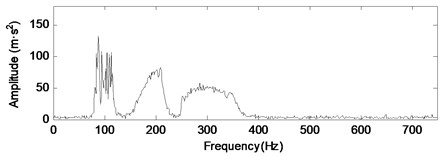
b)

In order to further analyze the signal, the simulation signal is decomposed by the VMD optimized by IAGA. In the IAGA, the population size is 8, and the evolution subalgebra is 100. In the process of IAGA optimization of modal number $K$ and penalty factor $\alpha$, the curve of the best fitness values in each generation is shown in Fig. 4.

Fig. 4The curve of the best fitness values in each generation

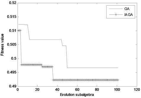
As shown in Fig. 4, the best fitness value of the proposed method appears in the 36th generation, and the best fitness value of the traditional genetic algorithm appears in the 50th generation. In comparison, the proposed method converges faster and inhibits the precocious phenomenon. After the end of evolution, the optimal parameters obtained by the proposed method are $\left(K,\alpha \right)=$ 3,646. Therefore, the modal number $K$ is set to 3, and the penalty factor $\alpha$ is set to 646. The simulation signal is decomposed by VMD, and the decomposition results are shown in Fig. 5.

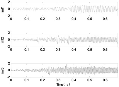
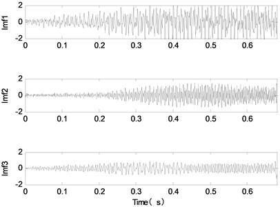
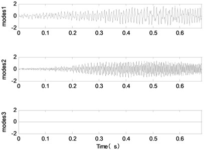
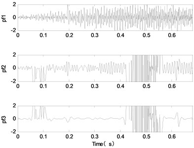
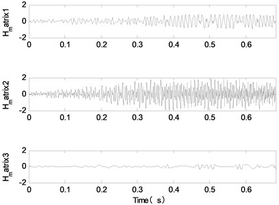
As shown in Fig. 5, the time domain waveform of the component of VMD decomposition is in good agreement with the time domain waveform of the signal source signal. That is to say, the proposed method has achieved good decomposition effect. In addition, in order to verify the advantages of the proposed method, EMD, EEMD, CEEMDAN, LMD and ITD are used to decompose the simulation signal, as shown in Fig. 6.

The energy of the first three components accounts for more than 90 % of the total energy of the simulation signal, so the first three components were selected for analysis. By comparing the signal source component in Fig. 2 with the signal decomposition component in Fig. 5 and Fig. 6, we can tentatively judge that the effect of the proposed method is the best. In order to further compare the authenticity of the components obtained by different methods, correlation coefficient is used as evaluation index. The correlation coefficients between the components decomposed by different methods and the simulation signal sources are compared, as shown in Table 1.

Fig. 5The decomposition results of the proposed method

Table 1Correlation between decomposition components and simulation signal source components

Decomposition methods	Component 1	Component 2	Component 3
VMD	0.99	0.99	0.98
EMD	0.85	0.73	0.86
EEMD	0.57	0.76	0.86
CEEMDAN	0.84	0.4	0
LMD	0.1	0.03	0.01
ITD	0.86	0.6	0.05

According to Table 1, it is easy to see that, compared with other methods, the components obtained by the proposed method are more closely related to the simulation signal source components. Thus, the components obtained by the proposed method are closer to the real signal, and the decomposition effect is the best.

5.2. Experiment condition

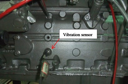
The structure of diesel engine is complex, and the working environment is abominable. As a result, it is prone to malfunction. The crankshaft bearing is located inside the engine, so it is difficult to diagnose the fault. In this paper, vibration signals are collected from the vibration sensors on the experimental stand, as shown in Fig. 7. The basic parameters of the vibration sensor are shown in Table 2. The engine on the experimental stand is Cummins 6BT diesel engine, and its parameters are shown in Table 3.

Table 2Vibration sensor parameters

Model	Sensitivity	Frequency range (±3 dB)	Range	Resolution	Temperature range	Weight	Output connector
603C01	100 mV/g	0.5 Hz-10 KHz	±50 g	350 μg	–54-121℃	51 g	Top

The fourth crankshaft bearings of Cummins EQ6BT diesel engine are set with different clearance (0.10 mm, 0.26 mm, 0.40 mm, 0.55 mm) to simulate the normal, slight, moderate and heavy wear of the crankshaft bearing. Vibration signals are collected on the left side of the fourth main bearings on the surface of the engine block. The sampling frequency is 20000 Hz and the sampling points are 4096 points.

Testing temperature is important when acquiring vibration signals. In the experiment, the temperature of cooling water is measured to reflect the internal temperature of diesel engine. The temperature is controlled at 60-70°C.

Table 3Basic parameters of the engine

Engine type	6BT5.9-G2	Fuel type	Diesel oil	Type	Inline 6 cylinders
Rated power (KW)	118	Compression ratio	17.5:1	Ignition sequence	153624
Rated speed (RPM)	2600	Continuous Power (KW)	86	Maximum torque (N·m)	558
Radius (mm) ×Distance (mm)	102×120	Maximum torque speed (r/min)		1600

Fig. 6The decomposition results of other methods

a) EMD

b) EEMD

c) CEEMDAN

d) LMD

e) ITD

Fig. 7Measuring position of vibration sensor

5.3. Data acquired

The acquisition system is composed of collector, computer, sensor and connecting circuit, as shown in Fig. 8. The acquisition system set the speed of the engine to 1800 r/min.

Fig. 8Vibration signal acquisition system

The vibration signals of the engine under different wear conditions are collected, as shown in Fig. 9. In Fig. 9, there is a large amount of background noise in the vibration signals of different wear conditions of the crankshaft bearing. The shock component of the signal is not obvious, and the fault feature cannot be extracted effectively.

5.4. Experimental data processing

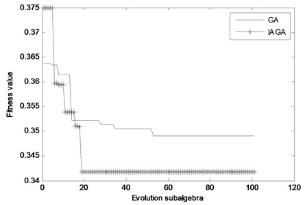
As an example, the slight wear signal of the crankshaft is analyzed by the method proposed. The vibration signal is decomposed by the VMD optimized by IAGA. In the IAGA, the population size is 8, and the evolution subalgebra is 100. In the process of IAGA optimization of modal number $K$ and penalty factor $\alpha$, the curve of the best fitness values in each generation is shown in Fig. 10.

As shown in Fig. 10, the best fitness value of the proposed method appears in the 19th generation, and the best fitness value of the traditional genetic algorithm appears in the 55th generation. In comparison, the proposed method converges faster and inhibits the precocious phenomenon. After the end of evolution, the optimal parameters obtained by the proposed method are $\left(K,\alpha \right)=$ 5,873. Therefore, the modal number $K$ is set to 5, and the penalty factor $\alpha$ is set to 873. The slight wear vibration signal is decomposed by VMD, and the decomposition results are shown in Fig. 11.

As shown in Fig. 11, the slight wear vibration signal is decomposed into 5 components by VMD. In the same way, the vibration signals of normal wear, moderate wear and heavy wear are decomposed into 5 components. In order to select the appropriate component as the fault component, the permutation entropy of each component under different wear states is calculated respectively, as shown in Table 4.

Fig. 9Vibration signals in different wear conditions

a) Normal wear

b) Slight wear

c) Moderate wear

d) Heavy wear

Fig. 10The curve of the best fitness values in each generation

As can be seen from Table 4, for different wear conditions, the entropy permutation value of the component $u_1$ is all minimal. That is, the randomness of the signal is minimal, and the shock component is the strongest. Therefore, the component $u_1$ is selected as the fault component. The spectrums of the component $u_1$ under different wear conditions are shown in Fig. 12.

Table 4The decomposition component permutation entropy of vibration signals under different wear conditions

Wear condition	$u_1$	$u_2$	$u_3$	$u_4$	$u_5$
Normal wear	0.38	0.42	0.56	0.61	0.64
Slight wear	0.36	0.42	0.57	0.69	0.67
Moderate wear	0.33	0.41	0.53	0.55	0.64
Heavy wear	0.30	0.41	0.56	0.62	0.65

Fig. 11The decomposition components of vibration signal under slight wear condition

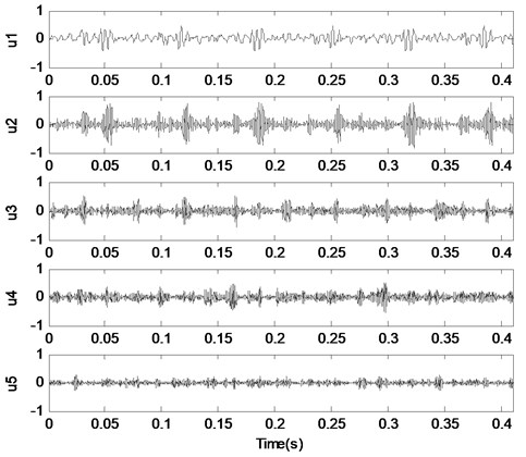
Fig. 12The decomposition components of vibration signal under slight wear condition

a) Normal wear

b) Slight wear

c) Moderate wear

d) Heavy wear

As can be seen from Fig. 12, the more serious the fault is, the greater the energy of the component $u_1$. In order to further analyze the fault components, the energy of the component $u_1$ under different wear conditions is extracted, as shown in Table 5.

As can be seen from Table 5, for the components obtained by VMD, the change of energy is not consistent with the wear fault of the crankshaft bearing. But for the fault component $u_1$, with the increase of the degree of wear, its energy is also increasing. Therefore, the component $u_1$ can be used as the characteristic component of the fault diagnosis of the crankshaft bearing wear, which is in agreement with the results of the previous permutation entropy. The wear fault diagnosis of the crankshaft bearing can be realized by monitoring the change of the energy of component $u_1$.

Table 5Basic parameters of the engine

Wear state	$u_1$	$u_2$	$u_3$	$u_4$	$u_5$
Normal wear	39.7	102.4	90.9	48.0	125.0
Slight wear	69.1	147.8	49.0	26.8	52.4
Moderate wear	141.4	193.8	85.9	136.1	97.9
Heavy wear	366.5	151.2	76.6	60.3	74.9

In order to accurately analyze the wear failure of diesel engine crankshaft bearing, 40 sets of components $u_1$ energy values are extracted as training samples for support vector machine (SVM), as shown in Table 6. In addition, other 40 sets of components $u_1$ energy values are extracted as test samples for SVM, as shown in Table 7. Specifically, 1, 2, 3 and 4 represents the normal, slight, moderate, and heavy wear of the crankshaft bearing respectively. The results of SVM’s training and test are shown in Fig. 13.

Table 6Training samples

Feature parameters	Fault type	Feature parameters	Fault type	Feature parameters	Fault type	Feature parameters	Fault type
38.7	1	76.4	2	153.8	3	350.0	4
45.6	1	71.2	2	153.4	3	374.6	4
40.1	1	71.2	2	223.4	3	357.2	4
41.4	1	71.6	2	215.3	3	349.8	4
40.6	1	73.4	2	222.8	3	343.9	4
40.1	1	77.0	2	223.1	3	402.0	4
38.3	1	76.5	2	222.3	3	357.8	4
40.9	1	73.6	2	222.4	3	338.8	4
40.9	1	73.4	2	218.1	3	350.6	4
39.4	1	75.1	2	211.3	3	367.1	4

Table 7Test samples

Feature parameters	Fault type	Feature parameters	Fault type	Feature parameters	Fault type	Feature parameters	Fault type
43.1	1	70.3	2	150.4	3	388.8	4
45.1	1	75.7	2	165.6	3	346.3	4
39.6	1	71.4	2	203.5	3	353.2	4
39.8	1	70.2	2	201.8	3	347.5	4
39.5	1	69.6	2	216.3	3	407.2	4
40.0	1	74.5	2	163.9	3	371.6	4
99.7	1	76.5	2	212.9	3	356.1	4
39.6	1	74.0	2	206.3	3	345.9	4
38.3	1	71.0	2	155.9	3	350.6	4
44.0	1	74.9	2	156.8	3	358.0	4

As can be seen from Fig. 13, the recognition rate of the test set sample reached 97.5 %, and fault types can be effectively identified by SVM. Therefore, the proposed method has achieved good diagnostic results. For the diagnosis of other diesel engines, a large number of confirmatory experiments are needed to make further research.

Fig. 13The training and test results of SVM

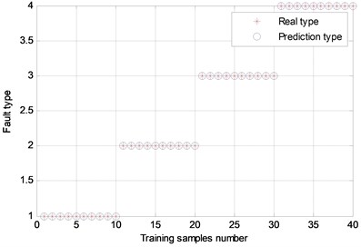
a) Accuracy rate 100 %

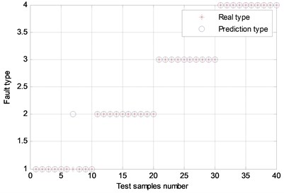
b) Accuracy rate 97,5 %

6. Conclusions

Aiming at the problem that VMD’s modal number $K$ and penalty factor $\alpha$ are difficult to be determined, an improved VMD algorithm based on adaptive genetic algorithm is proposed, which reduces the interference of human factors to decomposition results. The simulation signal and the fault diagnosis of diesel engine crankshaft are studied. The conclusions are as follows:

(1) In this paper, the crossover and mutation operators of traditional adaptive genetic algorithm are optimized, so that individuals maintain good diversity. Then the precocious phenomenon is avoided, and the problem of slow evolution is solved. VMD is optimized by IAGA, and the optimal parameter combination is obtained by the evolution of the population.

(2) As is known to all, mechanical fault diagnosis of diesel engine is difficult. According to the proposed method, the vibration signals under different wear conditions are studied, and the characteristic component of the wear fault of the diesel engine crankshaft bearing and its energy are effectively extracted. The wear fault of the diesel engine crankshaft bearing can be effectively identified by SVM, which provides a theoretical basis for the condition monitoring and fault diagnosis of the diesel engine crankshaft bearing wear.