Application of confidential intervals for verification of reservoir model at interpretation of well test data

1. Introduction

If information about the parameters of the formation before well testing, then information about these parameters from the point of view of Bayesian inference is expressed through a uniform probability distribution in the parameter space. The well test data contains the necessary information about the parameters, and the goal of analyzing the results of well test is to extract this information for use in updating the probability distributions in the parameter space. Confidence intervals can give a quantitative estimate of the information obtained [1].

Direct application of confidence intervals to the results of well test requires two conditions. First, the errors that represent the difference between the actual pressure value and its true value must be independent and normally distributed with respect to the true pressure change. The second condition is that for a domain in a parameter space sufficiently close to their estimates, the objective function can be approximated by a linear form by expanding it in a first-order Taylor series.

When these conditions are met, the updated probability distribution of unknown parameters generates a multidimensional normal distribution in the parameter space. A feature of the multidimensional normal distribution is that it is completely characterized by only two parameters: the mean value vector and the covariance matrix. For nonlinear regression analysis, the mean value vectors are parameter estimates, and the covariance matrix is calculated using the inverse Hesse matrix of the objective function on the basis of the final values of the estimates [2, 3].

2. The model of the system

The condition that the function describing the model can be approximated by expanding it in a Taylor series of the first order leads to the following expression:

It is believed that the observed pressure readings are normally distributed with respect to the true value of $F\left(\theta ,x_i\right)$ with the known variance:

As a result of observations of pressure values, the likelihood function for the parameters has the form:

where:

OLS is equivalent to the maximum of the likelihood function, which takes place if and only if:

As a result:

The Hessian matrix in the Gaussian method, divided by 2, is defined as [2]:

Then:

If for parameters the locally uniform a priori probability distribution is used (non-informative a priori probability distribution), then by the Bayes theorem the posterior probability distribution of the parameters after the $n$ observations [1, 4]:

where $\mathrm{P}\mathrm{r}\mathrm{o}\mathrm{b}\left(\theta \right)$ is a locally uniform a priori probability distribution.

By the definition of the multidimensional normal distribution:

Therefore, the equation takes the form:

That is, the parameters $\theta$ form a multidimensional normal distribution with respect to $\widehat{\theta }$ with the covariance matrix ${\sigma }^2{\mathbf{H}}^{-1}$. Eq. (11) quantifies the uncertainty associated with the parameter estimates.

When variance ${\sigma }^2$ is unknown, the above reasoning requires a little refinement. ${\sigma }^2$ can be obtained from the mean square error $s^2$, which is calculated as:

where:

In this case $s^2$ is an unbiased estimate of ${\sigma }^2$, and ${\sigma }^2$ has an inverse gamma distribution with respect $s^2$ with $n-m$ degrees of freedom:

where $v=n-m$.

Since $\theta$ and ${\sigma }^2$ are independent random variables, $\widehat{\theta }$ does not change even when ${\sigma }^2$ is replaced by $s^2$.

As a result, a posteriori probability distribution for $\theta$ can be obtained by excluding ${\sigma }^2$ when integrating the total a posteriori probability distribution density for $\theta$ and ${\sigma }^2$:

After substituting Eqs. (11) and (14) into Eq. (15), we obtain:

Therefore, when ${\sigma }^2$ is unknown, the parameters $\theta$ form the multidimensional $t$ – distribution of the Student relative to $\widehat{\theta }$ with the covariance matrix $s^2{\mathbf{H}}^{-1}$ and $n-m$ degrees of freedom.

The marginal probability distribution of the parameter ${\theta }_j$ is determined by excluding ${\theta }_i$ ($i\ne j$, $i=$ 1,…, $m$) when integrating over the space $\theta$:

where ${\sigma }_{{\theta }_j}$ is the Standard deviation, defined as:

where $h_{jj}^{-1}$ is the $j$th diagonal element of the inverse Hessian matrix computed at the point.

The more information is received about the parameters based on well test, the narrower the probability distribution with the shorter tails becomes. Accordingly, marginal probability distributions narrow down. Confidence intervals are used to quantify the range of marginal probability distributions.

By definition, a 95 % confidence interval covers 95 % of the area under the probability density curve, i.e. It is a range, the confidence probability of getting parameter values inside which is 95 %. Since the probabilities are distributed according to the normal law, the corresponding marginal distributions of each parameter are symmetric with respect to the estimates of these parameters. This means that the 95 % confidence interval is also symmetric with respect to the parameter estimate.

Usually, there are two types of confidence intervals: the range of absolute values and the range of relative values. Relative values are obtained by dividing the absolute values by the value of the parameter estimate.

In cases where the variance ${\sigma }^2$ is unknown, the ($1-\alpha$)·100 % th confidence interval for each parameter is determined from the following inequality [1]:

where $t_{1-\alpha /2}$ is the table value of the quantile of the order 1 – $\alpha$/2 for the $t$ – Student’s distribution with $n-m$ degrees of freedom.

In cases where $n-m>$ 30, the value $t_{1-\alpha /2}$ can be replaced by the corresponding value for the normal distribution. So, for $\alpha =$ 0,05 its value will be equal. Then Eqs. (19) takes the form “$y$”:

The $\left(1-\alpha \right)\cdot$100 % th confidence interval for the relative values of each parameter is determined from the following inequality:

Similarly, when $n-m>$ 30, the confidence interval for the relative values of each parameter can be represented as:

The correlation coefficient between any two parameters is calculated on the basis of elements located outside the main diagonal of the inverse Hessian matrix, at the point $\theta =\widehat{\theta }$:

As long as there are mathematical correlations between the parameters, none of them can be uniquely determined.

The joint application of confidence intervals and correlation coefficients requires the construction of confidence areas. (1 – $\alpha$)·100 % th confidence area of parameters is defined as follows:

where $F_{1-\alpha }\left(m,n-m\right)$ is a tabulated quantile value of the order $1-\alpha$ for $F$ – distribution with $m$ and $n-m$ degrees of freedom.

For the convenience of the use of confidence intervals in the verification of the model, the variance of the probability distribution is taken into account, and not the correlation between the parameters. In practice, the values of the confidence intervals: ±10 % for permeability $k$, coefficient of accumulation $C$, distance to the border ($r_e$), crack length ($x_f$); ±20 % for coefficient of elastic capacity $\omega$, transmittance $\lambda$; ±1 for skin factor $S$ and ±0.005 MPa for initial pressure ($P_i$). They were obtained heuristically on the basis of real experiments on the interpretation of field and simulated well test data.

The key idea is that if the model is chosen correctly and there is enough data, then all parameters should be within these acceptable limits. In this case, it is assumed that the model is selected correctly. Otherwise, the model is considered unacceptable, since confidence intervals exceed statistically allowable limits.

The variance of the probability distribution of each parameter is the product of the product of the mean square error and the corresponding diagonal element of the inverse Hessian matrix.

The mean square error is used to represent the variance of errors, which has a finite value, provided that a suitable model is selected. If this condition is met, then the mean square of the errors does not depend on the number of data and the time interval of well test. However, in the case of an incorrect model, the mean square of the errors becomes larger than the real value of the error variance.

The inverse Hessian matrix is a function of the number of parameters of the formation, which is equivalent to the dependence on the choice of the model, the correlation between the parameters, the amount of data and the time interval of well test. The property of the diagonal elements of the inverse Hessian matrix is that their values decrease monotonically with increasing amounts of data.

3. Computational experiments

Let’s demonstrate how confidence intervals can be used to assess the correctness of the model. For this purpose, the data of well test was modeled by the method of lowering the level. The purpose of the demonstration is to show how the confidence intervals solve the problem when it is known in advance whether the reservoir model corresponds to the data or not.

In the first case, the model was chosen correctly. The pressure values for well test by the method of level reduction were calculated using the flow model in an infinite formation, to which random errors were then added. Information on the reservoir and the fluid that saturates it: borehole radius $r_w=$ 0.1 m, reservoir thickness $h=$ 5 m, volume factor $B_o=$ 1 ${\left[m^3\right]}_{reservoir}/{\left[m^3\right]}_{norm}\text{,}$ viscosity $\mu =$ 10^-3 Pa·sec, porosity $\varphi =$ 0.2, initial pressure $P_i=$ 20 MPa, total compressibility $c_t=$ 10-4 MPa^-1, operating rate $q=$ 100 m³/day.

The true values of the parameters are $k=$ 0.05 µm², $S=$ 10 and $C=$ 0.2 m³/MPa. The random number generator generated a set of random errors distributed according to the normal law with zero mathematical expectation and variance 2.5·10^-5 MPa². Depending on the number of data points, the following four cases were considered: a) 51 data point, b) 61 data point, c) 71 data point and d) 81 data point. A flow model was used in an infinite reservoir with three parameters ($k$, $S$ and $C$). The correspondence of the model to the data is illustrated in Fig. 1.

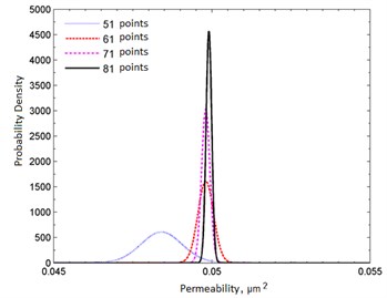
For simplicity, the results are given only for one parameter permeability. Marginal probabilities are shown in Fig. 2. The corresponding 95 % confidence intervals for permeability are summarized in Table 1.

Fig. 1Simulated well test data and its correspondence to the correctly chosen reservoir model

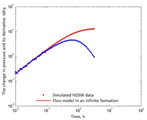
a) 51 points

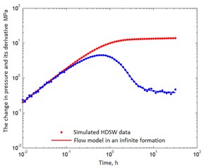
b) 71 points

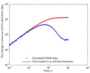
c) 61 points

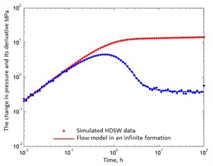
d) 81 points

In fact, only cases b), c) and d) contain useful information on permeability. As follows from Table 3, the permeability estimates are fairly close to the true value of 0.05 µm². Therefore, in Fig. 2 all probability distributions are grouped around this value. As the number of data increases, more permeability information appears, and the corresponding deviation (${\sigma }_{\theta }$) decreases. The spread of the distributions narrows, and the normal distribution tends to take the form of the Dirac delta function. From the standpoint of confidence intervals, all cases are acceptable, i.e. The model is chosen correctly.

Fig. 2Marginal densities of the probability distribution in the case of a correctly chosen reservoir model

4. Conclusions

In principle, confidence intervals can be used to accept or reject the selected model. Regardless of whether the model is chosen correctly or not, confidence intervals ultimately yield consistent results. But it must be taken into account that in practice, when verifying a model, confidence intervals should be determined for all parameters. In addition, confidence intervals are easy to calculate, since all the necessary information is contained in the results of nonlinear regression, and it is not difficult to use for model verification, as was demonstrated above.

However, comparative analysis based on confidence intervals has two drawbacks (practical and theoretical) from the standpoint of discriminant analysis of models.

First, the confidence intervals are directly proportional to the variance of the probability distribution of the parameter, which in turn is a combination of the mean squared error (estimated variance) $s^2$ and the diagonal element of the Hesse inverse matrix $h_{jj}^{-1}$. That is, confidence intervals can be in acceptable redistributions, even if an incorrect model is used.

Secondly, confidence intervals are convenient for verification of models, but are not suitable for their discriminant analysis. In other words, based on confidence intervals, you can determine whether the model is suitable or not, but nothing can be said about which of the models is better. This is due to the fact that the correlation between parameters is not taken into account when calculating confidence intervals. However, in general, reservoir parameters are nonlinearly related to each other, which must be taken into account when verifying. Moreover, Eq. (11) indicates that the dimension of the probability distribution of the parameters coincides with their number. That is, different models with different number of parameters have different dimensions of probability distributions. Therefore, a direct comparison of the corresponding confidence intervals is clearly not enough.