Abstract
Reliability bench tests and probability design method are two important means to improve the reliability of machine tools, while the load spectrum of machine tools is the foundation of reliability bench tests and probability design. According to the load spectrum, the actual working conditions can be simulated in laboratories. A dynamic load spectrum generation method is proposed to establish a representative load spectrum. Firstly, the cutting load measuring system is established based on the characteristics of the cutting loads, and then the actual cutting experiments designed by the orthogonal experimental method are conducted on the basis of the typical cutting conditions in laboratories. Secondly, the counting method of the cutting loads cycles is presented based on the dynamic load characteristics of a machining center. And loads cycles are counted by the proposed counting method, and then a rainflow matrix is formed. Thirdly, in order to improve the precision of the load spectrum the extrapolation of the loads is carried out using the parametric extrapolation method. Then the probability distribution functions of the mean and amplitude of the cutting loads are provided by the K-S goodness-of-fit test method. The case study indicates that the radial force, axial force, and cutting torque of the tested machining center follow gamma, normal, and Weibull distributions with different parameters, respectively. Finally, the joint distribution function of the mean and amplitude of the radial force, axial force, and cutting torque is obtained by using a combination of statistical analysis method, and the two-dimensional load spectrum of the MC is compiled.
1. Introduction
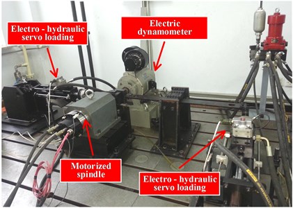
A machining center (MC) is a high-tech machine tool and regarded as measuring a country’s comprehensive national strength and industrial modernization. In recent years, the gap between domestic (China) and foreign MCs in machining accuracy, machining speed, multi-axis movement and process complexity has been shortened gradually, while in regard to the reliability, there still exists considerable disparity, especially for those equipped with domestic functional units [1-3]. The inherent reliability of products is primarily determined by design, so the main method to improve the reliability is to conduct reliability design. A MC is a complex system consisting of mechanical, electrical, hydraulic, pneumatic subsystems and other subsystems. However, the probability design theory is not stable and mature enough for the complex system. So, conducting reliability tests become a primary approach to improve the reliability of products. Most kinds of potential failures can be stimulated by reliability bench tests and subsequently conduct reliability evaluation, failure analysis, and finally improve design. As shown in Fig. 1, it is a motorized spindle reliability bench test [1] and it can simulate the actual working conditions of MCs. As known from engineering experience, cutting loads of a MC is determined by cutting parameters, both of which are selected purpose-oriented by machine tool users. Under this circumstance, the working conditions of the field tests become uncontrollable. Meanwhile, because of the long testing period, it is difficult to update the testing conditions and the needs of products synchronically. Thus, reliability bench tests become the research hotspot. One problem for reliability bench tests is how to develop a high precision load spectrum.
Fig. 1Motorized spindle reliability bench test
The process of developing dynamic load spectrum for MCs includes selecting typical cutting processes, acquisition of load data, extrapolating load spectrum and compiling load spectrum. Load data are the bases of load spectrum. A few scholars have investigated about load acquisition for mechanical products and obtained lots of achievements in the automobile, construction machinery and aviation industries [4-6]. B. Oelmann [7] conducted 20 measurements annually to determine the driveline loads in the actual driving processes. D. S. Milčić [8] used measuring stripes LY 12 to obtain the torque on a working wheel shaft depending on the operating regime of the bucket wheel excavator. Jeongho Oh [9] conducted cluster analysis using a classification distribution to develop a load spectrum for statewide axles. D. N. Kolonius [10] simulated the movements of machine tools to predict bearing capacity and actual loads through a computer simulation program, but the extreme loads were not predicted for some parameters limitation. Jürgen Fleischer [11] simulated the motions of machine tools using the multi-body dynamics method to obtain the virtual load spectrum of machine tools. Then he developed a reliability evaluation model with considering the effects of machine tools loads.
MCs, which are the foundation of manufacturing equipment, are widely used in the mechanical industries. Load spectrum generation methods have been studied by various scholars to improve the reliability of machine tools. In the late 1990s, Shen Guixiang and Wang Yiqiang et al. [12] collected the cutting parameters through the field tests and established a static load spectrum through the cutting load empirical formulas. But the loads obtained by the empirical formulas are static, which ignored the dynamic loads generated during the actual cutting. According to the fatigue damage theory, dynamic loads are the main causes for the fatigue failures and random failures of products [13]. Thus, the static cutting load spectrum is no longer suitable for reliability bench tests of machine tools nowadays.
Considering the influence of the dynamic loads, we propose a dynamic load spectrum compilation method for MCs. In order to understand the actual load characteristics of MCs, the actual cutting experiments designed by the orthogonal experimental method are conducted in the laboratory. Then, cutting loads cycles are counted by the rainflow counting method to form a rainflow matrix after load signals preprocessing. The extrapolation of the cutting loads is carried out using the parametric extrapolation method, and then the parameters of the dynamic load spectrum are developed by the local-best particle swarm optimization (PSO) method. Finally, the two-dimensional load spectrum of MCs is compiled.
2. Cutting load cycles counting
Cutting loads of MCs are irregular and random in the actual cutting processes. Since, these loads change over time under the cutting conditions. To our knowledge, cycle counting is the most commonly used statistical counting method, in which load time history is measured through the accumulation of full-load cycles and half-load cycles.
2.1. Rainflow cycle counting theory
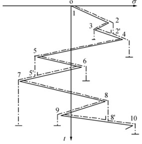
The rainflow counting algorithm is a two-parameter counting method developed by M. Matisuiski and Endo. This algorithm is used to extract load cycles from a load history, which can be obtained by measurement or simulation [15]. The rainflow cycle counting theory is described as follows:
1) Load-time history is assumed as a multistory roof turned clockwise by 90°, as shown in Fig. 2.
2) Water flows from its upper top on each of the “pagoda roofs” until one roof extends to the opposite side beyond the vertical of the starting point or the flow reaches a wet point.
3) When water reaches a peak, it drops to the next roof and stops until it meets another flow. Then, a full cycle is formed. Otherwise, a half cycle is generated.
4) Some rainflow cycles can be obtained according to the start and termination positions of flows. Then, the values of peaks and troughs of each cycle are extracted.
Fig. 2Rainflow cycle counting theory
2.2. Load cycle counting by the rainflow cycle counting theory
Data compression and cycle extraction from load signals are conducted before rainflow counting. Data compression is a process of converting the original load signals to an array of which elements are valid amplitudes by distinguishing the peaks and troughs of the original load signals. During the extraction of load cycles, only the first value of load signals is considered to be valid when two or more of the same values exist. Also, there is an extracting rule for the inflection point. If the value of the inflection point is greater than its adjacent values, then it is considered as the maximum value and needs to be extracted. In order to improve the efficiency, the four-point cycle counting method is applied. Firstly, , , , are four consecutive points extracted from the load signals. Then, a full load cycle is defined as follows:
After the full load cycles are defined, the two middle points, which are not peaks or troughs, need to be removed. Then two new points are selected, and these four new points are assessed by using Eq. (1). If assessment results are inconsistent with Eq. (1), the first picking point is removed, and the next new point is selected. This process is repeated until all points are processed. The remaining points after the cycle extraction compose the half cycles.
The rainflow counting algorithm is applied off-line by using MATLAB to generate the full and half cycles intuitively, as illustrated in Fig. 3.
Fig. 3Simulation of rainflow counting in MATLAB
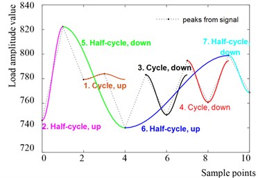
Load cycles can be classified as up cycles and down cycles respectively according to the changing directions of inflection points. Fig. 3 shows that section 1 is an up full cycle, sections 3 and 4 are two down full cycles, sections 2 and 6 are two up half cycles, and sections 5 and 7 are two down half cycles.
Results of the rainflow cycle counting are generally stored in a matrix to save memory space. Each load time history corresponds to a rainflow matrix containing mean and amplitude information. The is expressed as follows:
where represents the number of load cycles under the th level of the mean and th level of the amplitude.
If a rainflow matrix is divided into columns and rows, the results can be presented in a matrix table, which is called a 2-D load spectrum (Table 1).
Table 1Cycle frequency of different means and amplitudes of loads
Cycle frequency | Amplitude | ||||||
1 | 2 | ||||||
Mean | 1 | ||||||
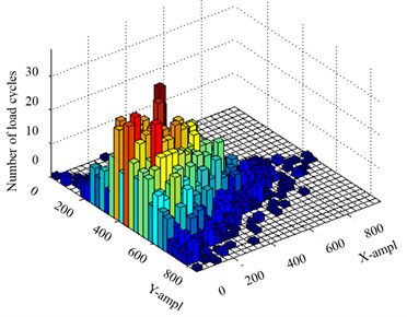
The load cycles versus the mean and amplitude can also be expressed by a histogram to provide a direct description (Figs. 4-6).
A large amount of loads that cause minimal or no damage to MCs is called invalid amplitude. Invalid amplitudes occupy a substantial space and would reduce the test efficiency. Thus, they should be eliminated. In this study, a dynamic threshold range model is selected to remove invalid amplitudes:
where is the threshold range, is the maximum, is the minimum of the loads, and represents the precision of the dynamic threshold range model, which is usually 10 %.
Fig. 4Histogram of the load amplitudes
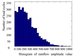
Fig. 5Histogram of the load means
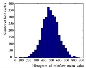
Fig. 6Three dimensional joint histogram of the means and amplitudes
3. Load preprocessing
3.1. Decomposition of cutting force
Assuming that the cutting force of each cutter tooth is applied to a single point at the same time, so the resultant cutting force can be divided into the main cutting force , passive force , and feed force . The decomposition of cutting force is shown in Figs. 7 and 8. The main cutting force is also called circular force; whose direction is the same as the main cutting movement. The torque , which is applied to a spindle, is the product of the main cutting force and tool radius. The passive force is the spindle axial force that is parallel to the axis of the spindle.
Fig. 7Three dimensional graphics of a face milling cutter
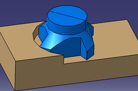
Fig. 8Decomposition of milling force
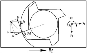
Thus, the passive force has a significant influence in both of the machining accuracy and surface roughness. The feeding force is the spindle radial force, which is perpendicular to the axis of the spindle. The tool handle bends easily and vibrates severely when the feeding force is high. Therefore, the parameter of feeding force is the basic consideration to verify the stiffness of a feed system.
Considering the structure and installation of a dynamometer, the cutting force are divided into three mutual perpendicular directions (, , and ) in a machine coordinate system, which are the orthogonal force components , and and they are shown in Fig. 8.
3.2. Regeneration of radial force in the time domain
The , , and are the cutting forces measured through the cutting tests, while and are the forces which are required to develop a load spectrum. Thus, Thus, an equivalent transformation method is applied to obtain the cutting force and from , , and . According to the force interaction principle, is equal to and other force components satisfy the following equation:
So, the radial force can be calculated by Eq. (4), while axial force and cutting torque can be measured directly by a dynamometer. Figs. 9-11 illustrate the actual waveforms of the radial force, axial force, and cutting torque in the time domain under one typical working condition.
Fig. 9Actual waveform of the radial force in the time domain

Fig. 10Actual waveform of the axial force in the time domain

Fig. 11Actual waveform of the cutting torque in the time domain

3.3. Sectional processing of the cutting force
A complete cutting process includes three sections, which are processes of cutting in (), cutting (), and cutting out (). Fig. 12 shows that the cutting force fluctuates seriously in different cutting processes. Although and contribute a small proportion of the entire process, the amplitude changes significantly in these two stages, particularly in . Extreme loads are usually generated when the cutting tool comes in contact with a workpiece during . Recent studies show that extreme loads would result in tool fracture and workpiece damages. But during , the load amplitudes change smoothly without evidently increasing or decreasing. Results are different during the period , the load amplitudes decrease at first but increase subsequently within a short time until the cutting tool finishes retraction.
Fig. 12Load waveform in different cutting processes

Limited by the size of the sample tested in laboratories, the proportion of the three cutting processes is inconsistent with the actual situations. For example, the proportion of obtained in the cutting tests is smaller than the actual one, thus, should be extrapolated on the basis of the actual cutting parameters. Statistical analysis reveals that and account for 2 % respectively and contributes 96 % of the whole cutting process. Then, the database of should be extended proportionally. Since is a static cutting process which consists of a series of equivalent small cutting period, the extension has a minimal effect on the whole loading distribution. Thus, in the case of constructing load spectrum, the factors above should be considered.
4. Parametric extrapolation method
4.1. Establishment of the distribution model
4.1.1. Cutting load cycle counting
Normalization is conducted before processing the cutting data. Therefore, the relative cutting force is expressed as follows:
where is the relative amplitude (or mean), is the amplitude (or mean), and is the maximum amplitude (or mean).
In each set, the ratio between the cycles corresponding to the relative amplitude (or mean) and the total cycles is the frequency which corresponding to the relative amplitude (or mean). The probability density function of a relative mean (or amplitude) can be expressed as follows:
where is the number of cycles corresponding to each relative amplitude (or mean), is the total number of cycles, and is the group interval of the relative amplitude (or mean).
If the values of amplitude (or mean) are superimposed in the three periods of , , and respectively, the accumulative probability density values of the sample could be obtained as:
4.1.2. Parameter estimation and goodness of distribution fitting
Distributions models of two-parameter Weibull distribution, lognormal distribution, and gamma distribution are considered as alternative distribution functions to develop the optimal model for the load spectrum. Data of the mean (or amplitude) are fitted to each alternative distribution function, of which parameters are estimated by the local-best PSO method. Then the goodness of distribution fitting is conducted to test the assumed underlying distributions by the statistical goodness-of-fit method. There are many statistical tools that can help in deciding whether or not a distribution model is a good choice from a statistical point of view. To find a best fit curve, a normalized RMS error (NRMSE) is obtained by dividing RMSE [16] by the average, which can be expressed as:
where is the number of groups, is the actual value of the probability density function, and is the fitting value of the probability density function.
The goodness-of-fit test is performed via a K-S test method to verify the fitting effect. Define as the test statistic, which is expressed as:
where is the given significance level and can be found in the K-S critical value table.
can be calculated on the basis of . The null hypothesis is accepted when . Otherwise, the hypothesis should be rejected. Among all the alternative distribution models, the model with the minimum value of is considered as the best distribution model.
4.2. Two-dimensional joint distribution function of the loads
If two random variable and are mutually independent, both and follow the relationship illustrated below:
According to Fischer theorem, if two random variables and are mutually independent, then the chi-square follows the distribution with degrees of :
where is the sample size ofthe loads, is the grade number of the amplitude of the loads, is the grade number of the mean of the loads, denotes the cycles whose amplitudes are within class , refers to the cycles, whose means belong to class , denotes the cycles whose amplitudes are within class , whereas the means belong to class .
5. Application example
Spindle speed , feed rate , cutting depth , and cutting width are selected as experimental factors, and the experimental program is optimized by the orthogonal test method. A four-level table of the orthogonal test (Table 3) is established according to the cutting parameters listed in Table 2 which is obtained from the field tests.
Cutting tests were conducted in laboratory on the basis of the cutting parameters listed in Table 3. As shown in Fig. 13, the cutting force was measured by a Kistler dynamometer (Type: 9257B). Then the measured cutting load signals were input into a computer through the charge amplifier (Type: 5017B) and the data acquisition system (Type: 5697A1). Finally, the cutting force in the three directions were analyzed by the rainflow counting method and the results are shown in Figs. 14-18.
Table 2Actor-level table of the orthogonal test
Factor | Spindle speed (r/min) | Feed rate (mm/min) | Cutting depth (mm) | Cutting width (mm) |
1 | 450 | 200 | 0.5 | 6 |
2 | 1100 | 400 | 1 | 14 |
3 | 1750 | 600 | 1.5 | 22 |
4 | 2400 | 800 | 2 | 30 |
Table 3Four-level table of the orthogonal test
Num | Spindle speed (r/min) | Feed rate (mm/min) | Cutting depth (mm) | Cutting width (mm) |
1 | 450 | 200 | 0.5 | 6 |
2 | 450 | 400 | 1 | 14 |
3 | 450 | 600 | 1.5 | 22 |
4 | 450 | 800 | 2 | 30 |
5 | 1100 | 200 | 1 | 30 |
6 | 1100 | 400 | 0.5 | 22 |
7 | 1100 | 600 | 2 | 14 |
8 | 1100 | 800 | 1.5 | 6 |
9 | 1750 | 200 | 1.5 | 14 |
10 | 1750 | 400 | 2 | 6 |
11 | 1750 | 600 | 0.5 | 30 |
12 | 1750 | 800 | 1 | 22 |
13 | 2400 | 200 | 2 | 22 |
14 | 2400 | 400 | 1.5 | 30 |
15 | 2400 | 600 | 1 | 6 |
16 | 2400 | 800 | 0.5 | 14 |
In order to find the cutting force distribution rules, Weibull, LogNorm and Gamma are selected as three alternative distribution models. We apply the PSO method to estimate parameters of these alternative distribution models. Thereafter, the distribution model is verified through the goodness-of-fit test method. Results are shown in Figs. 14-18 and the parameters for the three alternative distribution models are shown in Table 4.
Fig. 13Cutting load measuring system
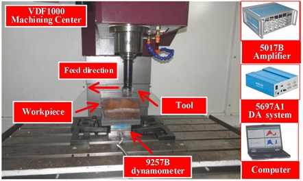
Table 4 shows that the amplitude of the radial force is in accordance with the gamma distribution at 3.09, 139.1. The mean of the radial force is consistent with the normal distribution at 454.3, 149.2. The amplitude of the axial force is in line with Weibull distribution at 335.8, 2.16. The mean of the axial force is in agreement with the normal distribution at 268.1, 96.3. The amplitude of the cutting torque is also consistent with Weibull distribution at 36.4, 2.07. The mean of the cutting torque is also in accordance with Weibull distribution at 22.2, 2.49.
Fig. 14Histogram of radial force amplitude value
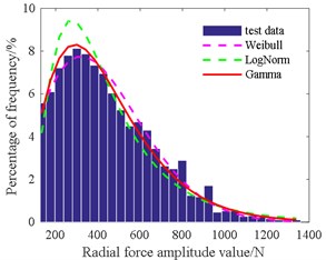
Fig. 15Histogram of radial force mean value
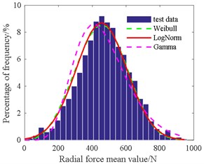
Fig. 16Histogram of axial force amplitude value
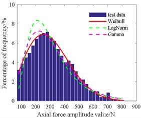
Fig. 17Histogram of axial force mean value
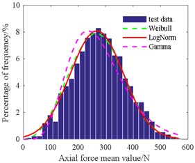
Fig. 18Histogram of cutting torque amplitude value
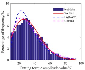
Fig. 19Histogram of cutting torque mean value
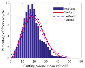
Table 4Parameter and K-S test results for the three alternative distribution models
Force | Index | DIST | PRM 1 | PRM 2 | Index | PRM 1 | PRM 2 | ||
Radial | AMP | Weibull | 475.4 | 1.90 | 0.03 | Mean | 505.8 | 3.44 | 0.013 |
LogNorm | 5.93 | 0.56 | 0.03 | 454.3 | 149.2 | 0.007 | |||
Gamma | 3.09 | 139.1 | 0.02 | 8.36 | 55.4 | 0.03 | |||
Axial | AMP | Weibull | 335.8 | 2.16 | 0.01 | Mean | 300.7 | 3.12 | 0.02 |
LogNorm | 5.61 | 0.50 | 0.05 | 268.1 | 96.3 | 0.01 | |||
Gamma | 3.62 | 83.9 | 0.03 | 7.07 | 38.8 | 0.03 | |||
Torque | AMP | Weibull | 36.4 | 2.07 | 0.01 | Mean | 22.2 | 2.49 | 0.02 |
LogNorm | 3.38 | 0.52 | 0.05 | 19.4 | 8.5 | 0.03 | |||
Gamma | 3.22 | 10.3 | 0.03 | 4.71 | 4.3 | 0.03 | |||
0.24 | |||||||||
According to Eq. (11), we obtain that 213.5. Considering that:
So . In conclusion, the cutting force mean, and amplitude are mutually independent when 0.05, and the two-dimensional joint probability density functions of the radial force, axial force, and torque are expressed as follows:
For the purpose of facilitating the application of the load spectrum to the reliability bench tests and simulating the actual working conditions, a continuous probability density distribution is adapted into a two-dimensional program load spectrum. The 8-step ladder curve is used to carry out the loading test. The amplitude is divided into 8 levels by unequal interval (ratio coefficient: 1, 0.95, 0.85, 0.725, 0.575, 0.425, 0.275, and 0.125). Thus, a two-dimensional load spectrum of the cutting load amplitudes is formed. The two-dimensional (amplitude-mean) program load spectrum of the radial force is shown in Table 5. The cumulative reliability test time is 1100.52 h.
Table 5Two-dimensional (amplitude-mean) program loading spectrum of radial force
Grade | Mean / | Amplitude / | |||||||
1 | 2 | 3 | 4 | 5 | 6 | 7 | 8 | ||
147 | 265 | 469 | 670 | 871 | 1055 | 1206 | 1307 | ||
1 | 59 | 1.13 | 1.52 | 1.22 | 0.68 | 0.29 | 0.09 | 0.02 | 0.02 |
2 | 177 | 5.97 | 8.04 | 6.44 | 3.61 | 1.55 | 0.48 | 0.13 | 0.12 |
3 | 295 | 17.68 | 23.81 | 19.09 | 10.68 | 4.59 | 1.41 | 0.39 | 0.35 |
4 | 413 | 62.62 | 84.33 | 67.59 | 37.83 | 16.27 | 5.00 | 1.37 | 1.23 |
5 | 531 | 88.64 | 119.37 | 95.68 | 53.55 | 23.03 | 7.07 | 1.94 | 1.74 |
6 | 649 | 55.86 | 75.23 | 60.30 | 33.75 | 14.52 | 4.46 | 1.22 | 1.10 |
7 | 767 | 16.22 | 21.84 | 17.51 | 9.80 | 4.21 | 1.29 | 0.35 | 0.32 |
8 | 885 | 1.35 | 1.82 | 1.46 | 0.82 | 0.35 | 0.11 | 0.03 | 0.03 |
6. Conclusions
The load spectrum of machine tools is the foundation to conduct probability design and reliability bench tests. With the application of the rainflow cycle counting method, a new strategy of generating dynamic load spectrum is developed to resolve the inconformity between the field tests and the reliability bench tests because of the lack of the dynamic load information.
1) The cutting load measuring system is built and then the 16 sets of cutting tests are designed by the orthogonal test method.
2) In order to improve the precision of the load spectrum, the extrapolation of the load is carried out by the parametric extrapolation method. The results reveal that the probability distribution functions of the radial force obey to gamma distribution with 3.09, 139.1. The mean of the radial force is consistent with the normal distribution at 454.3, 149.2. The amplitude and mean of the axial force are in line with Weibull distribution at 335.8, 2.16 and the normal distribution at 268.1, 96.3, respectively. The amplitude and mean of cutting torque are consistent with Weibull distribution at 36.4, 2.07 and 22.2, 2.49, respectively.
3) The joint distribution function of the mean and amplitude of the radial force, axial force, and torque are obtained by using a combination of statistical analysis methods, and the two-dimensional program loading spectrum of MCs is compiled.
The next step we will conduct reliability bench tests of the key function units of machine tools according to the two-dimensional program load spectrum. The generated equivalent load spectrum can be easily reproduced on a test bench for verifying and approving the reliability of MCs. It is of great significance to improve reliability level of MCs.
References
-
Yang Z. J., Chen C. H., Chen F., et al. Progress in the research of reliability technology of machine tools. Chinese Journal of Mechanical, Vol. 20, 2013, p. 130-139, (in Chinese).
-
Zhang J. H., Zhang S. G., Zhao H. X., et al. Structure design and test for guide unloading system of large ultra-precision machine. Optics and Precision Engineering, Vol. 9, 2007, p. 1383-1390, (in Chinese).
-
Yang Z. J., Chen C. H., Chen F., et al. Reliability analysis of machining center based on the field data. Eksploatacja i Niezawodnosc – Maintenance and Reliability, Vol. 15, Issue 2, 2013, p. 147-155.
-
Wang Y., Zhu C. Load spectrum modeling for tracked vehicles based on variational Bayesian inference. Proceedings of the Institution of Mechanical Engineers Part B Journal of Engineering Manufacture, Vol. 229, Issue 1, 2015, p. 178-188.
-
Kwon J. H., Joo S. Y., Hwang K. J., et al. Load spectrum generation using probabilistic random process and fatigue life prediction for automobile muffler structure. International Forum on Strategic Technologies, 2008, p. 53-57.
-
Carboni M., Cerrini A., Johannesson P., et al. Load spectra analysis and reconstruction for hydraulic pump components. Fatigue and Fracture of Engineering Materials and Structures, Vol. 31, Issue 31, 2008, p. 251-261.
-
Oelmann B. Determination of load spectra for durability approval of car drive lines. Fatigue and Fracture of Engineering Materials and Structures, Vol. 25, Issue 12, 2002, p. 1121-1125.
-
Milčić Dragan S., Miladinović Slobodan M., Mijajlović Miroslav M., et al. Determination of load spectrum of bucket wheel excavator SRS 1300 in coal strip mine drmno. Transactions of Famena, Vol. 37, Issue 1, 2013, p. 77-88.
-
Oh J., Walubita L. F., Leidy J. Establishment of statewide axle load spectra data using cluster analysis. KSCE Journal of Civil Engineering, Vol. 19, Issue 7, 2014, p. 1-8.
-
Kolonius D. N. Predicting the loading of machine tools. Machines and Tools, Vol. 5, 1991, p. 10-12.
-
Fleischer Jurgen, Wieser Jan, Schopp Matthias, et al. availability increase of machine tools through adapted maintenance activities and assembly-specific maintenance intervals. 15th CIRP International Conference on Life Cycle Engineering: Conference Proceedings, 2008, p. 388-393.
-
Wang Y. Q., Shen G. X., Jia Y. Z. Multidimensional force spectra of CNC machine tools and their applications, part one: force spectra. International Journal of Fatigue, Vol. 25, 2002, p. 1037-1046.
-
Chen C., Tian H., Zhang J., et al. Study on failure warning of tool magazine and automatic tool changer. Journal of Vibroengineering, Vol. 18, Issue 2, 2016, p. 883-899.
-
Lv Z. Q., Peng W. W., Huang H. Z. improved data processing of loading spectrum for applications of rainflow counting method. Journal of Donghua University, Vol. 32, Issue 6, 2015, p. 919-922.
-
Li Y., Xu M., Wei Y., et al. An improvement EMD method based on the optimized rational Hermite interpolation approach and its application to gear fault diagnosis. Measurement, Vol. 63, 2015, p. 330-345.
Cited by
About this article
Our deepest gratitude goes first to the editors and reviewers for their constructive suggestions on the paper. In addition, thank the authors of this paper’s references whose work have contributed greatly to the completion of this thesis. Second, we would like to thank National Natural Science Foundation-Youth Foundation (51505186), National Natural Science Foundation of China (Grant No. 51675227), China Postdoctoral Science Foundation (No. 2015M580245), Science Research Plan of Jilin Province ([2015]472), Jilin Province Excellent Researcher Foundation (20170520103JH) and Jilin Province Science and Technology Development Funds (20160204006GX).
Chuanhai Chen and Zhaojun Yang conceived the idea of load spectrum for machining center; Hailong Tian conducted the majority of the experimental work, Jialong He discussed the results; Shizheng Li and Chuanhai Chen wrote the manuscript; Dongliang Wang analyzed the experimental data; Zhaojun Yang edited the manuscript and checked grammatical and spelling errors.
