Fault detection and diagnosis of rotating machinery using modified particle filter

Li, Ke; Liu, Yiya; Wu, Jingjing; Su, Lei; Chen, Peng

doi:10.21595/jve.2017.18078

Journal of Vibroengineering

Browse Journal

Submit article

Published: 15 August 2017

Check for updates

Fault detection and diagnosis of rotating machinery using modified particle filter

Ke Li¹

Yiya Liu²

Jingjing Wu³

Lei Su⁴

Peng Chen⁵

^{1, 2, 3, 4}Jiangsu Key Laboratory of Advanced Food Manufacturing Equipment and Technology, Jiangnan University, 1800 Li Hu Avenue, Wuxi, Jiangsu, 214122, China

^{5, 1}Graduate School of Bioresources, Mie University, Mie, 514-8507, Japan

Corresponding Author:

Jingjing Wu

Cite the article Download PDF

Downloads 1747

WoS Core Citations 1

CrossRef Citations 1

Abstract

In order to effectively monitor condition and detect fault types of high nonlinear system, and extract the features of system state under strong noise background, this paper proposes a novel fault detection and diagnosis (FDD) method based on modified particle filter (PF). The artificial neural network is incorporated in PF for adaptively adjusting weight of particle. In the modified PF, the large weight particles are split into several small weight particles, the particles with smaller weight is adjusted by using artificial neural network. By which the particles in the low probability density region are adjusted to the high probability density region, and the problem of particle leanness is solved effectively. Moreover, this paper also uses time-varying auto regressive (TVAR) and Akaike information criterion (AIC) methods to establish state space model for state estimation. Finally, the proposed method is implemented for fault diagnosis on a roller bearing. Good results are obtained, and the bearing faults, such as the outer race, the inner race and the roller element defects, have been effectively discriminated.

1. Introduction

Fault detection and diagnosis (FDD) have vast importance to improve production efficiency, ensure production safety, and reduce maintenance costs of plant. FDD based on vibration analysis techniques are most common and effective method, which are widely used in mechanical fault diagnosis and condition monitoring. However, due to the complexity of the plant structure and the noise interference in the work locale, the vibration signals measured for mechanical fault diagnosis and condition monitoring are highly nonlinear, and often contain stronger noise components [1-3]. The information that can reflect mechanical condition is buried via noise components. In these cases, mechanical status cannot be effectively detected, and even may lead to misrecognition. Therefore, how to effectively remove the noise and extract the features of the fault signals are very important for mechanical fault diagnosis and condition monitoring.

Many studies based on vibration signal processing technology for mechanical fault diagnosis purpose have been carried out. Signal filtering techniques based on Fourier transform have been the dominating signal processing tool for condition diagnosis [4-9], and widely applied in engineering practice. Sadly, Fourier transform has some limitations, such as the signal to be processed must satisfy periodicity and stationary requirements. Thus, Fourier transform is not applicable to nonstationary or nonlinear signals, and unable to reveal the intrinsic features of nonstationary and nonlinear signals [10, 11]. Wavelet Transform (WT) is a power tool for analyzing nonstationary signals, and has become a hot spot in the research of modern signal processing. WT method shows a good picture in the joint time-frequency domain, and clearly describe the change of frequency vary with time. In [12] the discrete WT was used to decompose the vibration signal of the rolling bearing, and spalling failure of rolling bearing was successfully predicted online. In [13] wavelet packet and support vector machine were integrated to detect faults of a rolling bearing. However, the results of signal de-noising largely depend on the selection of wavelet basis functions. Only selecting the appropriate basis function, the features of signal can be well to detect. In addition, because of the limited length of the wavelet basis function, the leakage of signal energy is inescapable. Kalman filter is an optimal recursive data processing algorithm, which often be used to estimate system state for linear systems with Gaussian noise. In [14] a Kalman filter based on the methodology of the maximum likelihood estimation was established, by which sensor fault was correctly estimated. Reference [15] used Kalman filter to predict the future state, so as to realize the preventive maintenance of DC motor. In order to extend Kalman filter to the nonlinear system, extended Kalman filter (EKF) [16] and unscented Kalman filter (UKF) [17] were proposed. However, when the system is strongly nonlinear, filtering accuracy of these improved Kalman filter will be greatly reduced, and even lead to output divergence of system filtering.

PF is recursive Bayesian filtering estimation based on sequential Monte Carlo algorithm. It is a nonlinear filtering method, and provides an effective way to solve the state estimation of nonlinear system under non Gauss noise. In the last decade, PF has been widely applied in many fields, such as tracking problem, mobile robot navigation, mechanical fault diagnosis and machinery life prediction [18-23]. In [19] authors combined PF with $M$ -algorithm, by which sensor faults were detected accurately and effectively. In [20] authors proposed a new PF based on genetic operator’s algorithm, which called intelligent PF. This method was used for fault diagnosis of a nonlinear system, and got good results. In [21] PF and UKF method were integrated for FDD, and two numerical examples verified the effectiveness of this method.

In the fault diagnosis of rotating machinery, the vibration response is obviously nonlinear due to the changes of stiffness, friction, fault excitation and external excitation and so on. Multiple vibrations are coupled to each other and fault characteristic signal is buried under strong noise background. Although the traditional PF can be used as an effective means to solve the nonlinear problem, but the algorithm still has some problems. The traditional PF suffer from a loss of diversity among particles after resampling and cannot accurately characterize posterior probability density. To solve FDD of high nonlinear system, and extract the features of machinery state under strong noise background, this paper proposes a novel FDD method based on modified PF. The artificial neural network is incorporated in PF for adaptively adjusting weight of particle, by which the particles in the low probability density region are adjusted to the high probability density region, and the problem of particle leanness is solved effectively.

The structure of this paper is organized as follows, Section 2 introduces the theory of the general PF, and expounds the problem in the general PF; In Section 3, the modified PF based on artificial neural network is described detailed, and the example that commonly used in PF testing is presented; In Section 4, the practical example of mechanical fault diagnosis for a bearing is designed to verify the effectiveness of the proposed method, and we also compared the proposed method with the WT technique. Section 5 summarizes and concludes this paper.

2. Theory of particle filter

PF is recursive Bayesian filtering estimation based on Monte Carlo algorithm [24]. The essence of PF is to approximate the posterior probability density by a set of weighted random samples.

In general, the system of state equation and measurement equation can be expressed as:

1

x_{t} = f_{t} (x_{t - 1}) + ω_{t - 1},

2

z_{t} = h (x_{t}) + ε_{t},

where, $x_{t}$ express the system state variable at time $t$ , and $z_{t}$ is the observed value of $x_{t}$ at time $t;$ $ω_{t}$ and $ε_{t}$ indicate system noise and measurement noise, respectively; $f (\cdot) :$ $R^{n_{x}} \times R^{ω_{x}} \to R^{n_{x}}$ indicates state transition function, and $h (\cdot)$ : $R^{n_{x}} \times R^{ε_{x}} \to R^{n_{z}}$ expresses the measurement function.

The recursive Bayesian filtering includes two steps: prediction and updating.

Prediction:

3

p (x_{t}| z_{1 : t - 1}) = \int p (x_{t} |x_{t - 1}, z_{10 : t - 1}) p (x_{t - 1}| z_{1 : t - 1}) d x_{t - 1} = \int p (x_{t} |x_{t - 1}) p (x_{t - 1}| z_{1 : t - 1}) d x_{t - 1} .

Updating:

4

p (x_{t}| z_{1 : t}) = \frac{p (x_{t}| z_{1 : t - 1}) p (z_{t}| x_{t})}{p (z_{t}| z_{1 : t - 1})},

where:

5

p (z_{t}| z_{1 : t - 1}) = \int p (x_{t} |z_{1 : t - 1}) p (z_{t}| x_{t}) d x_{t} .

For non-linear and non-Gaussian systems, it is difficult to obtain posterior probability $p (x_{t}| z_{1 : t})$ by the analytic solution. Therefore, the sequential importance sampling (SIS) method is applied in PF. SIS algorithm transforms integral operation into sum operation of samples, and approximates the state posterior probability density by a set of weighted particles ${\{x_{0 : t}^{i}, ω_{t}^{i}\}}_{i = 1}^{N}$ that sampled from an importance probability density function. The posterior probability $p (x_{0 : t}| z_{1 : t})$ at time $t$ can be approximated by the particles as follows:

6

p (x_{0 : t} | z_{1 : t}) = \sum_{i = 1}^{N} ω_{t}^{i} δ (x_{0 : t} - x_{0 : t}^{i}),

where, $N$ is the number of the particles.

The importance probability density function:

7

q (x_{0 : t}| z_{1 : t}) = q (x_{t}| x_{t - 1,}, z_{t}) q (x_{0 : t - 1}| z_{1 : t - 1}) .

The weight $ω_{t}^{i}$ for each particle:

8

ω_{t}^{i} = \frac{p (x_{0 : t} | z_{1 : t})}{q (x_{0 : t} | z_{1 : t})} \propto ω_{t - 1}^{i} \frac{p (z_{t}| x_{t}^{i}) p (x_{t}^{i}| x_{t - 1}^{i})}{q (x_{t}^{i}| x_{0 : t - 1}^{i}, z_{1 : t})},

where, the symbol $\propto$ indicates to be proportional to.

The normalized weight ${\tilde{ω}}_{t}^{i}$ is:

9

{\tilde{ω}}_{t}^{i} = \frac{ω_{t}^{i}}{\sum_{i = 1}^{N} ω_{t}^{i}} .

The posterior probability $p (x_{0 : t}| z_{0 : t})$ is rewritten as:

10

p (x_{0 : t} | z_{1 : t}) = \sum_{i = 1}^{N} {\tilde{ω}}_{t}^{i} δ (x_{0 : t} - x_{0 : t}^{i}),

where, $δ (\cdot)$ is Dirac-delta function.

The state $x_{t}$ can be estimated as:

11

{\hat{x}}_{t} \approx \sum_{i = 1}^{N} {\tilde{ω}}_{t}^{i} x_{t}^{i} .

In SIS，after a few iterations, most of particles have negligible weights, PF algorithm occurs particle degeneracy [25]. To deal with the particle degeneracy problem, this study adopts multinomial resampling technique, and its procedure is shown in Table 1.

Table 1Multinomial resampling

Step 1: For

i =

1, 2, …,

N

, draw a sample set

\{u_{i}\}

from the uniformly distribution (0, 1]

Step 2: For

i =

1, 2, …,

N

, find the variable quantity

j

(

j =

1, 2, …,

N

) that satisfies

\sum_{n = 1}^{j - 1} ω_{n} < u_{i} \leq \sum_{n = 1}^{j} ω_{n} .

Step 3: Store the

x_{t}^{i}

as a new particle, and the weight of the new particle

ω_{t}^{i} =

1/

N

The degree of particle degeneracy can be appraised using the effective sample size $N_{e f f}$ [26]:

12

N_{e f f} = \frac{1}{\sum_{i = 1}^{N} ({\tilde{ω}}_{t}^{i})^{2}} .

From Eq. (12), the smaller value of the effective sample size $N_{e f f}$ , the more serious the problem of particle degradation will be. Setting the threshold of effective sample $N_{r}$ , $N_{r} = m \times N$ , $m \in$ (0, 1). If $N_{e f f} < N_{r}$ particle degradation is serious, PF system performs resampling. After resampling process, the particles that have small weight are knocked out, and many new particles are obtained by the particles that have big weight, as shown in Fig. 1. The procedure of PF is presented as Table 2.

Table 2The procedure of PF

Step 1: Set time

t =

0, for

i =

1, 2,…,

N

, draw the particles

x_{0}^{i}

from the prior probability density, and all of the particles have same weight 1/

N

Step 2: For

i =

2, 3,…,

N

, draw the particles

x_{t}^{i}

from the importance probability density, calculate and normalize the particles weight

ω_{t}^{i}

by Eqs. (8) and Eq. (9)

Step 3: Calculate the effective sample size

N_{e f f}

. If

N_{e f f} < N_{r}

, resampling is carried out, the new particle set

{\{x_{0 : t}^{j}\}}_{j = 1}^{N}

is produced. If

N_{e f f} < N_{r}

, PF go to step 4, directly

Step 4: Estimate the state by Eq. (11)

Step 5: Set

t =

t

+1, and obtain the new measurement data, return to step (2)

Fig. 1Illustration of resampling

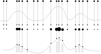
In resampling procedure, only the particles that have big weight are selected as copy samples, the new particles are replicas of them, and the particles with small weight are eliminated. In most cases, all the resampling operations are focused on a few particles with big weight, the particles lose diversity. This problem is also called particle leanness. The simple method to solve particle leanness problem is to increase the number of particle. However, computing burdens of PF will be increased. If computing time of PF is too long, PF is difficult to be applied in practical engineering.

For above the problems, this study proposed a novel PF algorithm based on BPNN, which is described in the next section.

3. Modified particle filter based on NN

In this section, an improved PF which is named AWPF is presented. The inspiration of this method is from back propagation neural network (BPNN).

3.1. Brief of BPNN

BPNN is a kind of multi layer feed-forward network which is trained by the error back propagation algorithm, and consist of input layer, hidden layer and output layer [27]. The gradient descent method is used to adjust the weight and threshold between each layer of BP-NN, to minimize sum of the squared errors. Let input data is $a_{i}$ ( $i =$ 1, 2,…, $N$ ), and corresponding teacher data is $x_{i}$ ( $i =$ 1, 2,…, $N$ ), $y_{i}$ is actual output. The network error function is as follows:

13

E = \frac{1}{2} \sum_{i = 1}^{n} (x_{i} - y_{i})^{2} .

The weight adjustment function is as Eq. (15):

14

Δ w_{i j} = - η \frac{\partial E}{\partial w_{i j}},

where, $η$ is learning rate of BPNN; $w_{i j}$ indicates the weight between each layer; $Δ w_{i j}$ expresses modified quantity of the weight.

3.2. AWPF

In AWPF algorithm, abruption and adjustment of particle weight are two basic and important operations, which are described as follows.

Particles abruption:

(1) Obtain the particles $x_{t}^{i}$ , $i =$ 0, 1,…, $N$ from the importance posterior probability density, and calculate the particles weight $ω_{t}^{i}$ by Eq. (8), and normalize the particles weight ${\tilde{ω}}_{t}^{i}$ by Eq. (9);

(2) Divide all of the particles into large weight particles and small weight particles by the strategy instructed as follows:

15

x_{t}^{i} \in \{\begin{array}{l} \begin{array}{l} N_{b}, & {\tilde{ω}}_{t}^{i} \geq R, \end{array} \\ \begin{array}{l} N_{s}, & {\tilde{ω}}_{t}^{i} < R, \end{array} \end{array}

where, $N_{b}$ and $N_{s}$ are large weight and small weight particle sets, respectively; $R$ is a threshold for separating the particles.

(3) Split every large weight particle in set $N_{b} {\{x_{t}^{i}, {\tilde{ω}}_{t}^{i}\}}_{i = 1}^{p}$ into two new particles, and the new particles weights equal to half of the before.

(4) After step (3) the number of particle has been increased to $N + p$ . In order to keep the number of particle unchanged, $p$ particles with the minimum weight in set $N_{s}$ are eliminated.

Weight adjustment:

(1) Sort the particles with the weight values in descending order;

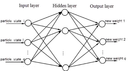
(2) Select $q$ particles with the minimum weight, and adjust their weights by using BPNN. The network error function is:

16

ε = \frac{1}{2} \sum_{i = 1}^{q} (z_{i} - y_{i})^{2} = \frac{1}{2} \sum_{i = 1}^{q} (e_{k})^{2},

where, $q$ is the number of input and output unit of the BPNN; $z_{i}$ is the measurement value, and used as teacher data; $y_{i}$ is output of the BPNN.

Fig. 2 is the BPNN diagram for PF algorithm. In Fig. 2, the input units are the state values of the particle with the minimum weight, and the corresponding weight of the particles are used as the initial weights of BPNN, the output units are the new particle weight values after adjustment, the number of hidden layer is set to eight.

After particles abruption and weight adjustment steps, the particles in the low probability density region are adjusted to the high probability density region, and the particle diversity is increased. The flowchart of AWPF is shown in Fig. 3.

Fig. 2BPNN diagram for PF algorithm

3.3. Simulation

In order to verify the effectiveness of AWPF, an example that commonly used in PF testing is presented, and described as follows:

17

x_{t} = 0.5 x_{t - 1} + \frac{25 x_{t - 1}}{1 + (x_{t - 1})^{2}} + 8 c o s 1.2 (t - 1) + ω_{t - 1},

18

y_{t} = 0.05 (x_{t})^{2} + v_{t},

where, $ω_{t - 1}$ is state noise, and $ω_{t - 1} ~ (N, σ_{w}^{2})$ ; $v_{t}$ is measurement noise, and $v_{t} ~ (N, σ_{v}^{2})$ ; in present test, $σ_{w}^{2}$ and $σ_{v}^{2}$ are 0.1 and 0.01, respectively; initial probability density function $p (x_{o}) ~ N (0,2)$ ; the number of the particle is set to 1000. This model is strong nonlinear and bimodal.

Root mean square error (RMSE) as shown in Eq. (20) is chosen to estimate the performance of AWPF:

19

R M S E = \sqrt{\frac{1}{n} \sum_{i = 1}^{n} (x_{i}^{} - {\hat{x}}_{i}^{})^{2},}

where $x_{i}$ is the simulation data. ${\hat{x}}_{i}^{}$ indicates estimate data. $n$ expresses length of the data.

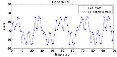
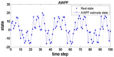
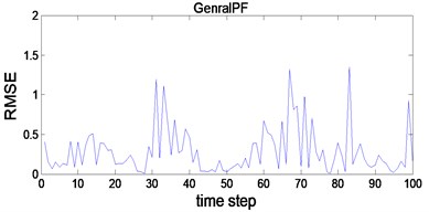
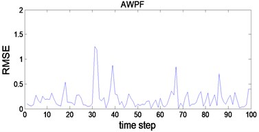
The simulations for the general PF and AWPF are performed on same test condition. Fig. 4 and Fig. 5 show the state estimate results and RMSE curve of the general PF and AWPF, respectively. Comparison of simulation data is listed in Table 3. As shown in Table 3, the mean accuracy of the general PF and AWPF are 0.568 and 0.292, the available samples of the general PF and AWPF are 192 and 405, respectively. The mean accuracy and the available samples of AWPF are greater than the general PF. That is to say AWPF can improve particle diversity and state estimate accuracy.

Fig. 3flowchart of AWPF

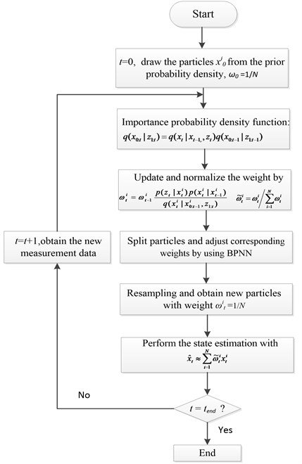
Fig. 4State estimate results using general PF and AWPF

a)

b)

Fig. 5RMSE curve of general PF and AWPF

a)

b)

Table 3Comparison of simulation

	Mean accuracy	Available samples
PF	0.568	192
AWPF	0.292	405

4. Application to Fault Detection

4.1. Experimental System

In this section, the performances of AWPF are verified via fault detection of a rolling bearing. In order to better interpretation of the performances of AWPF, WT method is introduced for comparison.

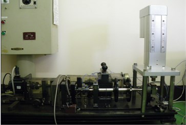
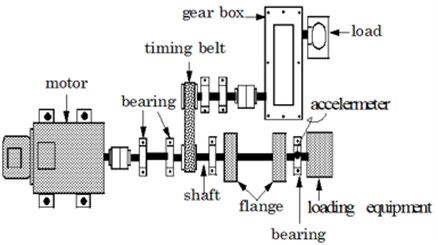
Fig. 6 shows the experimental platform for fault detection and diagnosis of a rolling bearing. As shown in Fig. 6, the power of the experimental platform is provided by a servo motor (Mitsubishi HG-SR352BJ), with output power 3.5 kW, rated speed 3000 rpm, rated voltage 380 V. The loading equipment (Shizuoka RCS2-RA13R) with 300 kg load is used to exert pressure on the rotating shaft. Two types of rolling bearing (N205 and NU205) are used for obtaining the vibration data of rolling bearing in each state. N205 that outer ring can be disassembled is used for normal, outer-race defect and roller element defect test. NU205 that inner-race can be disassembled is used for inner-race defect state. Fig. 7 shows the three kind of bearing faults, which are artificially processed by using Wire cutting machine, and fault width is 0.3 mm, and fault depth is 0.025 mm.

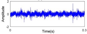
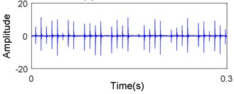
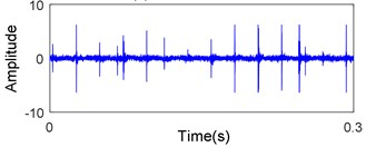
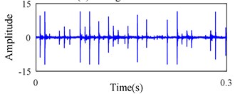
In present work, data acquisition system includes an accelerometer, signal conditioner, signal recorder and computer. The raw vibration signals are measured via the accelerometer at constant speed 1000 rpm, with 50 Hz sampling frequency. The sapling time is about 20 s. After amplified by the signal conditioner, the signals are transferred into the signal recorder. The raw signals measured in each state are shown in Fig. 8.

Fig. 6Illustrate of the experimental setup for test

a)

b)

Fig. 7Bearing defects: a) outer race defect, b) inner race defect, c) rolling defect

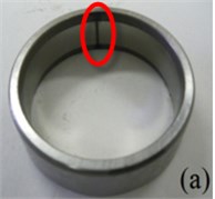
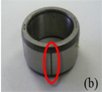
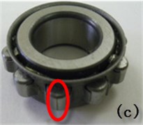
Fig. 8Raw vibration signals of the bearing

a) Normal

b) Outer-race defect

c) Inner-race defect

d) Rolling element defect

4.2. State-space model of vibration signal

4.2.1. State Equation

To use PF technique for FDD, the state model and measurement model described in Eqs. (1) and (2) need to be established firstly. Due to the complexity of mechanism and the diversity of mechanical failures, it is difficult to construct accurate vibration signal model. Thus, time-varying auto regressive (TVAR) method is used to construct the vibration signal model in this paper. Assuming $x_{t}$ is vibration signal, the TVAR model of vibration signal is as follows:

20

x_{t} = - \sum_{i = 1}^{p} a_{i} (t) x_{t - i} + e_{t},

where, $a_{i}$ indicates time-varying coefficient; $p$ denotes model order; $e_{t}$ is residual error of the model:

21

a_{i} (t) = - \sum_{j = 0}^{m} a_{i j} g_{j} (t),

where, $m$ is extended dimension; $a_{i j}$ is weight of basic function; $g_{j} (t)$ express time basic function. According to the vibration signal characteristic of rolling bearing, this study choice DCT basic function shown in Eq. (23) to estimate time-varying coefficient of TVAR model:

22

g_{j} (t) = a (t) c o s (\frac{j π (2 k + 1)}{2 N}),

23

a (t) = \{\begin{array}{l} \begin{array}{l} \sqrt{1 / N}, & t = 0, \end{array} \\ \begin{array}{l} \sqrt{2 / N}, & t \neq 0 . \end{array} \end{array}

Define:

24

A^{T} = [a_{10}, a_{11} \dots a_{1 m} \dots a_{p 0}, a_{p 1} \dots a_{p m}],

25

{X_{t}}^{T} = [x_{t - 1} g_{0} (t) \dots x_{t - 1} g_{m} (t) \dots x_{t - p} g_{0} (t) \dots x_{t - p} g_{m} (t)] .

According to least square principle, Eq. (21) can be rewritten as:

26

x_{t} = - X_{t}^{T} A + e_{t} .

Thus, the least square estimates of $A$ is:

27

\hat{A} = - {(\sum_{t = p + 1}^{N} X_{t} X_{t}^{T})}^{- 1} \sum_{t = p + 1}^{N} X_{t} x_{t} .

The least square estimates of the variance of $e_{t}$ :

28

{\hat{σ}}^{2} = \frac{1}{N - p} {\sum_{t = p + 1}^{N} [x_{t} + \sum_{i = 1}^{p} a_{i} (t) x_{t - i}]}^{2} .

In this paper, Akaike Information Criterion (AIC) method is introduced for determining model order $p$ , and mathematical expression of AIC is given as follows. A detailed description about AIC method can be found in reference [28]:

29

A I C (p) = l n {\hat{σ}}^{2} + \frac{2 p}{N - r},

where, $N$ is the length of signal; $r$ indicates pre-order of the model.

4.2.2. Measurement equation

Firstly, the original vibration signals measured by the accelerometer are decomposed into 5 layers by using WT with db1 wavelet function. Secondly, the threshold is extracted by ddencpm function. The wavelet coefficients that less than the threshold is retained, and the wavelet coefficients that greater than the threshold value are removed. Lastly, the remaining wavelet coefficients are reconstructed by the waverec function, and the reconstructed signal is the measurement noise.

Measurement equation:

30

z_{t} = x_{t} + w_{t},

where, $x_{t}$ and $z_{t}$ express state and measurement values at time $t$ , respectively; $w_{t}$ is measurement noise obtained by WT.

4.3. Calculation of characteristic frequency

Condition diagnosis of roller element bearing depends largely on analysing the vibration signals generated by localized defects. Fault types can be identified base on the characteristic frequencies which estimate by the geometry parameters of roller element bearing [29]. The characteristic frequencies of bearing defects can be calculated by the theoretical equation [30].

The characteristic frequencies of the outer race ( $f_{O}$ ):

31

f_{o} = \frac{1}{2} n f_{s} (1 - \frac{D_{B}}{D_{P}} c o s θ) .

The characteristic frequencies of the inner race ( $f_{I}$ ):

32

f_{I} = \frac{1}{2} n f_{s} (1 + \frac{D_{B}}{D_{P}} c o s θ) .

The characteristic frequencies of the roller ( $f_{E}$ ):

33

f_{E} = \frac{D_{P}}{D_{B}} f_{s} (1 - \frac{D_{B}^{2}}{D_{P}^{2}} c o s θ),

where $n$ is the number of balls in rolling elements bearing, $f_{r}$ indicates rotating frequency of motor, $D_{B}$ and $D_{P}$ are the ball diameter and the pitch circle diameter, respectively. $θ$ represents the bearing contact angle of roller bearing.

Above the characteristic frequencies are based on the ideal condition. However, in practice, some sliding motion may occur, which causes slight deviation of the characteristic frequency locations. In this work, the characteristic frequencies of the outer race defect, the inner race defect and the roller element defect are 88.76 Hz, 128.3 Hz, and 94.8 Hz, respectively.

4.4. Fault detection by the proposed method

Procedure of fault detection by AWPF is given as follows. Firstly, the vibration signals in each state are measured. Secondly, state-space models of the vibration signal are set up by the method ded in ion 4.2, and AWPF is used to estimate the probability density function of the system to achieve the purpose of vibration signal denoising. Thirdly, the envelope spectrum information s in each e were obtained. Finally, we detect the roller bearing state by the extracted spectra. Figs. 9-11 show parts of the verification results.

Fig. 9Signal of the out-race defect after AWPF

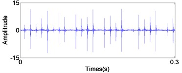
a) In time domain

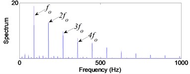
b) In frequency domain

Fig. 10Signal of the Inner race defect after AWPF

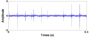
a) In time domain

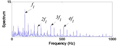
b) In frequency domain

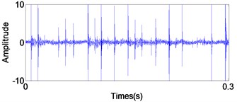
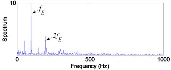
From Fig. 9(b), the impact repetition frequency $f_{O}$ is 89.8 Hz and its harmonics 2 $f_{O}$ , 3 $f_{O}$ and 4 $f_{O}$ are about 180.1 Hz, 270.2 Hz and 360.1 Hz, respectively. $f_{O}$ approaches the outer race defect characteristic frequency at 88.7 Hz that calculated by Eq. (20); therefore, we judge the fault type as the outer race defect. Similarly, in Fig. 10(b) the impact repetition frequency $f_{I}$ is about 129.7 Hz and its harmonics 2 $f_{I}$ , 3 $f_{I}$ and 4 $f_{I}$ are about 259.4 Hz, 387.6 Hz and 517.3 Hz, respectively. $f_{I}$ approaches the Inner race defect characteristic frequency at 128.3 Hz that calculated by Eq. (21); therefore, it was identified as the inner race defect by these spectra. On the basis of Fig. 11(b), the characteristic frequency $f_{E}$ is about 96.1 Hz, and close to the rolling element defect pass-frequency at 94.8 Hz that calculated by Eq. (22); its harmonics 2 $f_{E}$ is about 192.5 Hz. Although there are not any obviously characteristic at harmonics 3 $f_{E}$ and 4 $f_{E}$ , the rolling element defect of the bearing can be identified by the characteristic frequency $f_{E}$ and 2 $f_{E}$ .

As shown in Figs. 10 and 11, the repetition of harmonics and sidebands throughout the spectra of the inner race defect and the rolling element defect, which make the inner race and the roller defects are not easy to identify as the outer race defect. However, those defects can be identified by the corresponding bearing characteristic frequencies.

Fig. 11Signal of the roller element defect after AWPF

a) In time domain

b) In frequency domain

4.5. Fault diagnosis by traditional PF

In order to verify the effectiveness of the proposed method, several popular signal processing methods such as traditional PF, WT and Empirical Mode Decomposition (EMD) are used to compare with the proposed method in this paper.

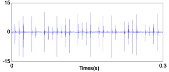
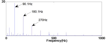
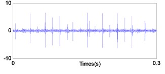
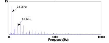
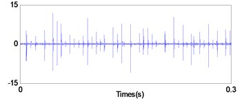
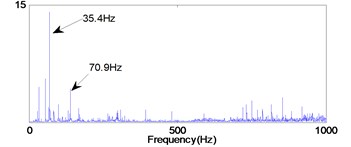
Figs. 12-14 show the diagnosis results by using traditional PF. From the Fig. 12 the impact repetition frequencies are 90.1 Hz, 180.1 Hz and 270 Hz respectively, and close to the characteristic frequency of the outer race defect and its harmonics. Hence, it was identified as the outer race defect. However, as shown in the Figs. 13 and 14, it is difficult to find the fault characteristic frequencies of inner race defect and rolling element defect.

Fig. 12Signal of the out-race defect after traditional PF

a) In time domain

b) In frequency domain

Fig. 13Signal of the inner race defect after traditional PF

a) In time domain

b) In frequency domain

Fig. 14Signal of the roller element defect after traditional PF

a) In time domain

b) In frequency domain

4.6. Fault diagnosis by wavelet transform

WT is a time-frequency signal analysis method, which can divide signal into different frequency regions and carry out signal decomposition and information extraction [31].

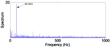
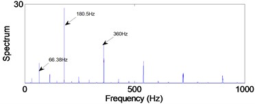
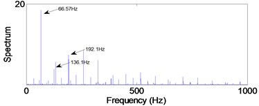
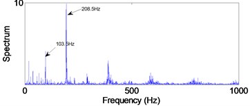
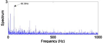
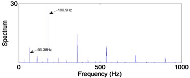
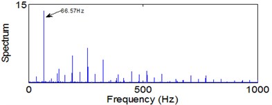
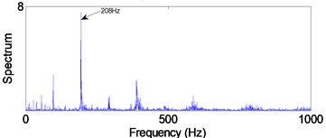
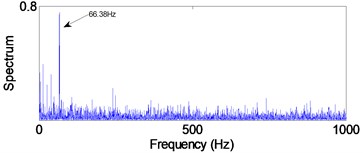
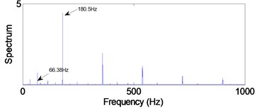
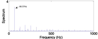
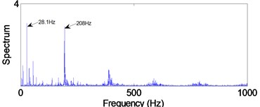
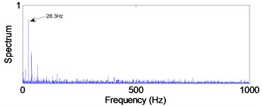
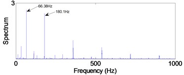
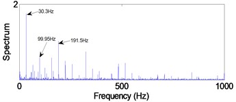
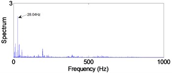
In this work, the wavelet function ReverseBior 2.8 is chosen for fault diagnosis, and diagnosis flowchart is as follows. Firstly, the raw signal measured in each defect state is decomposed into four levels in low-frequency regions (0-25 kHz, 0-12.5 kHz, 0-6.25 kHz and 0-3.125 kHz) and high-frequency regions (25-50 kHz, 12.5-25 kHz, 6.25-12.5 kHz and 3.125-6.25 kHz) by ReverseBior 2.8. Secondly, the signal components at each level are reconstructed in the time domain by reconstruction function. Lastly, the envelope spectra at each level are obtained by the FFT technique. The vibration caused by bearing defect is appeared in the high-frequency region generally. Hence, in present work we only analysis the signals in high-frequency levels. The envelope spectra of each high-frequency level are shown in Figs. 15-18. From the Figs. 15-18(b) the impact repetition frequency approaches to the twice outer race pass-frequency at about 180 Hz, they approach the twice outer race characteristic frequency 178 Hz, hence, it was identified as the outer race defect. However, as shown in the Figs. 15-18(c) and (d), it is difficult to find the fault characteristic frequencies of inner race defect and rolling element defect at each level, because the signal contains strong noise, the fault characteristic frequencies caused by the defective bearing and its harmonics are buried.

Fig. 15Envelope spectra in 25-50 kHz level

a) Normal

b) Outer-race defect

c) Inner-race defect

d) Rolling element defect

Fig. 16Envelope spectra in 12.5-25 kHz level

a) Normal

b) Outer-race defect

c) Inner-race defect

d) Rolling element defect

Fig. 17Envelope spectra in 6.25-12.5 kHz level

a) Normal

b) Outer-race defect

c) Inner-race defect

d) Rolling element defect

Fig. 18Envelope spectra in 3.125-6.25 kHz level

a) Normal

b) Outer-race defect

c) Inner-race defect

d) Rolling element defect

4.7. Fault diagnosis by EMD

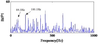
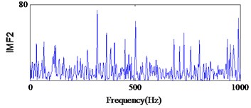
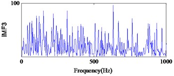
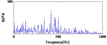
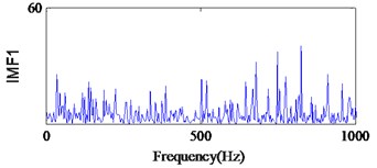
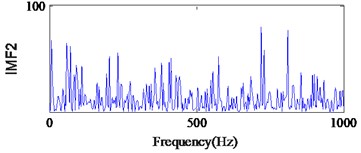
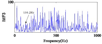
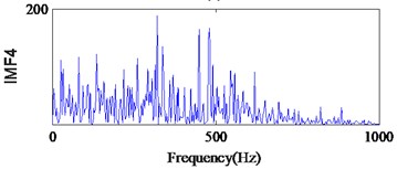
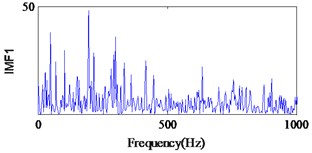
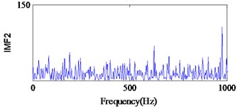
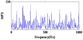
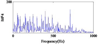
EMD is a non-stationary signal adaptive decomposition method proposed by Huang. According to the characteristics of the signal, EMD can adaptively select the frequency band, and determine the signal in different frequency resolution. In the last 10 years EMD has made great progress and has been successfully applied in mechanical fault diagnosis [32]. In this work, we also compare the proposed method with EMD method, and diagnosis procedure is as follows. Firstly, the vibration signal that measured in each state is decomposed into the different characteristic scale intrinsic mode function (IMF) by EMD. Secondly, the envelope spectra of each IMF are obtained by the FFT technique. Finally, the condition and fault type of the bearing are determined by analyzing envelope spectra of each IMF. As the high-frequency signal is distributed on the first few IMF components, in present work we only analysis the first four IMF components. The envelope spectra of IMFs in each state are shown in Figs. 19-21.

From Fig. 19(a), we can find the impact repetition frequency at about 89.3 Hz and 180.1 Hz, which approaches to the outer race defect characteristic frequency and the twice outer race defect characteristic frequency. Therefore, we judge the fault type as the outer race defect. Similarly, in Fig. 20(c) the impact repetition frequency at about 130.2 Hz can be find, and it approaches the Inner race defect characteristic frequency. Therefore, it was identified as the inner race defect by this spectrum. However, in Fig. 21 it is difficult to find the fault characteristic frequencies of the rolling element defect at each IMF.

Fig. 19Signal of the out-race defect after EMD

a)

b)

c)

d)

Fig. 20Signal of the Inner race defect after EMD

a)

b)

c)

d)

Fig. 21Signal of the roller element defect after EMD

a)

b)

c)

d)

On the basis of above verification results, three types bearing defects were effectively and accurately identified via the method proposed in this study. This shows that the method proposed in this study is the most efficacious for diagnosing bearing faults and eliminate much noise from the signal. Although the outer race defect of the bearing can be identified by using WT and traditional PF, it is difficult to identify the inner race and roller element defects. In add cation, the outer race and inner defects of the bearing can be identified with EMD method. However, the roller element defect cannot be identified, because the signal contains strong noise, the fault characteristic frequencies caused by the defective bearing and its harmonics are buried.

5. Conclusions

In order to effectively monitor condition and detect fault types of high nonlinear system, and extract the features of system state under strong noise background, this paper proposed a novel FDD method based on the modified PF which called AWPF. The BPNN was incorporated in PF for adaptively adjusting weight of particle. In AWPF, the large weight particles were split into two small weight particles, the particles with smaller weight was adjusted by using artificial neural network. By which the particles in the low probability density region were adjusted to the high probability density region, and particle diversity was increased. The problem of particle leanness was solved effectively. Moreover, TVAR and AIC methods were presented to establish state space model for state estimation. Finally, the proposed method was implemented for fault diagnosis on a roller bearing. We also compared the proposed method with traditional PF, WT and EMD techniques. The verification results shown that three types bearing fault had been effectively identified by the proposed method. However, these bearing faults were difficult to detect using traditional PF, WT and EMD techniques.

References

Jing L., Liangsheng Q. Feature extraction based on Morlet wavelet and its application for mechanical fault diagnosis. Journal of Sound and Vibration, Vol. 234, Issue 1, 2000, p. 135-148.

Publisher
Chen P., Toyota T., He Z. Automated function generation of symptom parameters and application to fault diagnosis of machinery under variable operation-conditions. IEEE Transactions on Systems, Man, and Cybernetics – Part A: Systems and Humans, Vol. 31, Issue 6, 2001, p. 775-781.

Publisher
Li K., Chen P., Wang S. M. An intelligent diagnosis method for rotating machinery using least squares mapping and a fuzzy neural network. Sensors, Vol. 5, 2012, p. 5919-5939.

Publisher
Pacas M., Villwock S., Dietrich R. Bearing damage detection in permanent magnet synchronous machines. Energy Conversion Congress and Exposition, Vol. 9, 2009, p. 1098-1103.

Publisher
Cheng J. S., Yu D. J., Yang Y. Application of an impulse response wavelet to fault diagnosis of rolling bearings. Mechanical Systems and Signal Processing, Vol. 21, Issue 2, 2007, p. 920-929.

Publisher
Randall R. B., Antoni J. Rolling element bearing diagnostics – a tutorial. Mechanical Systems and Signal Processing, Vol. 25, Issue 2, 2011, p. 485-520.

Search CrossRef
Bianchini C., Immovilli C., Cocconcelli M., Rubiniand R., Bellini A. Fault detection of linear bearings in brushless AC linear motors by vibration analysis. IEEE Transactions on Industrial Electronics, Vol. 58, Issue 5, 2011, p. 1684-1694.

Publisher
Stack J. R., Habetler T. G., Harley R. G. An amplitude modulation detector for fault diagnosis in rolling element bearing. IEEE Transactions on Industrial Electronics, Vol. 51, Issue 5, 2004, p. 1097-1102.

Publisher
Rajagopalan S., Restrepo J. A., Aller J. M., Habetler T. G., Harley R. G. Nonstationary motor fault detection using recent quadratic time-frequency representations. IEEE Transactions on Industry Applications, Vol. 44, Issue 3, 2008, p. 735-744.

Publisher
Randall R. B, Antoni J. Rolling element bearing diagnostics – a tutorial. Mechanical Systems and Signal Processing, Vol. 25, 2011, p. 485-520.

Publisher
Sheen Y. T. An analysis method for the vibration signal with amplitude modulation in a bearing system. Journal of Sound and Vibration, Vol. 303, Issue 3, 2007, p. 538-552.

Publisher
Mori K., Kasashima N., Yoshioka T., Ueno Y. Prediction of spalling on ball bearing by applying the discrete wavelet transform to vibration signal. Wear, Vol. 195, 1996, p. 162-168.

Publisher
Hu Q., He Z. J., Zhang Z. S., Zi Y. Y. Fault diagnosis of rotating machinery based on improved wavelet package transform and SVM ensemble. Mechanical Systems and Signal Processing, Vol. 21, Issue 2, 2007, p. 688-705.

Publisher
Wang Z. H., Shen Y., Zhang X. L. Attitude sensor fault diagnosis based on Kalman filter of discrete-time descriptor system. Journal of Systems Engineering and Electronics, Vol. 23, Issue 6, 2012, p. 914-920.

Publisher
Yang S. K. An experiment of state estimation for predictive maintenance using Kalman filter on a DC-motor. Reliability Engineering and System Safety, Vol. 75, Issue 1, 2002, p. 103-111.

Publisher
Ozbek L., Efe M. An adaptive extended Kalman filter with application to compartment models. communication in statistics-simulation and computation. Communications in Statistics – Simulation and Computation, Vol. 33, Issue 1, 2004, p. 145-158.

Publisher
Dias S. S., Bruno M. G. Cooperative target tracking using decentralized particle filtering and RSS sensors. IEEE Transactions on Signal Processing, Vol. 61, Issue 14, 2013, p. 3632-3646.

Publisher
Hiremath S. A., Van Der Heijden G. W., van Evert F. K., Stein A., Ter Braak C. J. Laser range finder model for autonomous navigation of a robot in a maize field using a particle filter. Computers and Electronics in Agriculture, Vol. 100, 2014, p. 41-50.

Publisher
Wei T., Huang Y. F., Philip Chen C. L. Adaptive sensor fault detection and identification using particle filter algorithms. IEEE Transactions on Systems, Man, and Cybernetics, Vol. 39, Issue 2, 2009, p. 201-213.

Publisher
Yin S., Zhu X. P. Intelligent particle filter and its application to fault detection of nonlinear system. IEEE Transactions on Industrial Electronics, Vol. 62, Issue 6, 2015, p. 3852-3861.

Search CrossRef
Liu Y., Sun D. Q., Kong L. Rao-blackwellized particle filtering for fault detection and diagnosis. Proceedings of the 29th Chinese Control Conference, 2010, p. 29-31.

Search CrossRef
Saha B., Goebel K., Poll S., Christophersen J. Prognostics methods for battery health monitoring using a Bayesian framework. IEEE Transactions on Instrumentation and Measurement, Vol. 58, Issue 2, 2009, p. 291-296.

Publisher
Aesarendra W. C, Niu G., Yang B. Machine condition prognosis based on sequential Monte Carlo method. Expert Systems with Applications, Vol. 37, Issue 3, 2010, p. 2412-2420.

Publisher
Doucet A., de Freitas N., Gordon N. Sequential Monte-Carlo Methods in Practice, Springer. New York, 2001.

Publisher
Douc R., Cappé O. Comparison of resampling schemes for particle filtering. Proceedings of the 4th International Symposium on Image and Signal Processing and Analysis, 2005, p. 64-69.

Publisher
Arulampalam M. S., Maskell S., Gordon N., Clapp T. A tutorial on particle filters for online nonlinear/non-Gaussian Bayesian tracking. IEEE Transactions on Signal Processing, Vol. 50, Issue 2, 2002, p. 174-188.

Publisher
Buscema M. Back propagation neural network. Substance Use and Misuse, Vol. 33, Issue 2, 1998, p. 233-70.

Publisher
Fei W. C., Bai L. Time-varying parameter auto-regressive models for autocovariance nonstationary time series. Science in China Series A: Mathematics, Vol. 52, Issue 3, 2009, p. 577-584.

Publisher
Tandon N., Choudhury A. A review of vibration and acoustic measurement methods for the detection of defects in rolling element bearings. Iribology International, Vol. 320, 1999, p. 469-480.

Publisher
Chen P., Toyota T. Sequential fuzzy diagnosis for plant machinery. JSME International Journal – Series C, Vol. 46, 2003, p. 1121-1129.

Publisher
Li K., Chen P., Wang H. Q. Intelligent diagnosis method for rotating machinery using wavelet transform and ant colony optimization. IEEE Sensors Journal, Vol. 12, Issue 7, 2012, p. 2474-2484.

Publisher
Li Y., Xu M., Wei Y., Huang W. An improvement EMD method based on the optimized rational Hermite interpolation approach and its application to gear fault diagnosis. Measurement, Vol. 63, 2015, p. 330-345.

Publisher

Cited by

Diagnostics and prognostics for complex systems: A review of methods and challenges

Morteza Soleimani | Felician Campean | Daniel Neagu

(2021)

About this article

Received

05 December 2016

Accepted

04 May 2017

Published

15 August 2017

SUBJECTS

Fault diagnosis based on vibration signal analysis

DOI

https://doi.org/10.21595/jve.2017.18078

Keywords

fault detection and diagnosis

particle filter

time-varying auto regressive

state estimation

Acknowledgements

The authors would like to acknowledge the financial support of the National Key Technology Support Program of China (2015BAF16B02), Fundamental Research Funds for the Central Universities (Grant No. JUSRP51732B and JUSRP51511).

Author Contributions

Ke Li, Peng Chen and Jingjing Wu conceived and designed the experiments; Ke Li and Peng Chen performed the experiments; Ke Li, Yiya Liu and Su Lei analyzed the data; Ke Li wrote the paper.

This is an open access article distributed under the Creative Commons Attribution License, which permits unrestricted use, distribution, and reproduction in any medium, provided the original work is properly cited.

Previous article in issue Previous Next article in issue Next

Review article

2021 11 26

Fault diagnosis and health management of bearings in rotating equipment based on vibration analysis – a review

Adnan Althubaiti, Faris Elasha, Joao Amaral Teixeira

Research article

2020 03 31

Fault diagnosis of rotating machinery under time-varying speed based on order tracking and deep learning

Taiyong Wang, Lan Zhang, Huihui Qiao, Peng Wang

Research article

2019 09 30

Bearing fault diagnosis based on feature extraction of empirical wavelet transform (EWT) and fuzzy logic system (FLS) under variable operating conditions

Fawzi Gougam, Chemseddine Rahmoune, Djamel Benazzouz, Boualem Merainani

Research article

2018 12 31

An intelligent fault diagnosis method of rotating machinery using L1-regularized sparse filtering

Weiwei Qian, Shunming Li, Jinrui Wang, Zenghui An, Xingxing Jiang

K. Li, Y. Liu, J. Wu, L. Su, and P. Chen, “Fault detection and diagnosis of rotating machinery using modified particle filter,” Journal of Vibroengineering, Vol. 19, No. 5, pp. 3395–3412, Aug. 2017, https://doi.org/10.21595/jve.2017.18078

Copy Extrica

Copied to clipboard!

TY  - JOUR
DO  - 10.21595/jve.2017.18078
UR  - https://doi.org/10.21595/jve.2017.18078
TI  - Fault detection and diagnosis of rotating machinery using modified particle filter
T2  - Journal of Vibroengineering
AU  - Wu, Jingjing
AU  - Li, Ke
AU  - Liu, Yiya
AU  - Su, Lei
AU  - Chen, Peng
PY  - 2017
DA  - 2017/08/15
PB  - JVE International Ltd.
SP  - 3395-3412
IS  - 5
VL  - 19
SN  - 1392-8716
ER  - 

Copy Ris

Copied to clipboard!

@article{Wu_2017,
	doi = {10.21595/jve.2017.18078},
	url = {https://doi.org/10.21595/jve.2017.18078},
	year = 2017,
	month = {aug},
	publisher = {{JVE} International Ltd.},
	volume = {19},
	number = {5},
	pages = {3395--3412},
	author = {Jingjing Wu and Ke Li and Yiya Liu and Lei Su and Peng Chen},
	title = {Fault detection and diagnosis of rotating machinery using modified particle filter},
	journal = {Journal of Vibroengineering}
}

Copy Bibtex

Copied to clipboard!

[1]J. Wu, K. Li, Y. Liu, L. Su, and P. Chen, “Fault detection and diagnosis of rotating machinery using modified particle filter,” Journal of Vibroengineering, vol. 19, no. 5, pp. 3395–3412, Aug. 2017, doi: 10.21595/jve.2017.18078.

Copy IEEE

Copied to clipboard!

Wu, Jingjing, Ke Li, Yiya Liu, Lei Su, and Peng Chen. “Fault Detection and Diagnosis of Rotating Machinery Using Modified Particle Filter.” Journal of Vibroengineering 19, no. 5 (August 15, 2017): 3395–3412. https://doi.org/10.21595/jve.2017.18078.

Copy Chicago

Copied to clipboard!

Fault detection and diagnosis of rotating machinery using modified particle filter

Abstract

1. Introduction

2. Theory of particle filter

3. Modified particle filter based on NN

3.1. Brief of BPNN

3.2. AWPF

3.3. Simulation

4. Application to Fault Detection

4.1. Experimental System

4.2. State-space model of vibration signal

4.2.1. State Equation

4.2.2. Measurement equation

4.3. Calculation of characteristic frequency

4.4. Fault detection by the proposed method

4.5. Fault diagnosis by traditional PF

4.6. Fault diagnosis by wavelet transform

4.7. Fault diagnosis by EMD

5. Conclusions

References

Cited by

About this article

Related Articles