Abstract
This paper is based on the experimental study for design and control of vibrations in automotive vehicles. The objective of this paper is to develop a model for the highly nonlinear Magneto-Rheological (MR) damper to maximize passenger comfort in an automotive vehicle. The behavior of the MR damper is studied under different loading conditions and current values in the system. The input and output parameters of the system are used as a training data to develop a suitable model using Genetic Algorithm. To generate the training data, a test rig similar to a quarter car model was fabricated to load the MR damper with a mechanical shaker to excite it externally. With the help of the test rig the input and output parameter data points are acquired by measuring the acceleration and force of the system at different points with the help of an impedance head and accelerometers. The model is validated by measuring the error for the testing and validation data points. The output of the model is the optimum current that is supplied to the MR Damper, using a controller, to increase the passenger comfort by minimizing the amplitude of vibrations transmitted to the passenger. Besides using this model for cars, bikes and other automotive vehicles it can also be modified by re-training the algorithm and used for civil structures to make them earthquake resistant.
1. Introduction
Isolation of the forces transmitted by external application is the most important function of a suspension system. The suspension system comprises of a spring element and a dissipative element, which when placed between the object to be protected and the excitation, reduces the vibration transmitted to the object. Suspension systems range from active to passive suspensions. MR damper lies in between this range and behaves like a semi-active suspension system. The damping of a passive suspension system is a property of the system and cannot be varied, whereas in an active suspension system the damping of the system can be altered by using an actuator to give it an external force. This external force helps in improving the ride quality. The shortcoming of this model is that it requires considerable amount of external power source, it is costly and is difficult to incorporate in the system due to the added mass. A variation of the active suspension system is the semi-active or the adaptive suspension system. In these systems, the damping of the system is varied by controlling the current thereby, changing the viscous properties of the damping elements in the suspension system. PID neural network controller, is one such controller used to develop a model to predict the displacement and velocity behavior of the MR damper [1]. In comparison to active suspension semi active suspension systems’ power consumption is considerably less. The magneto-rheological (MR) dampers and electro-rheological dampers are the most common examples of semi active dampers. In the past few years, research on MR dampers has improved its capabilities and reduced the gap between adaptive suspension system and truly active suspension systems. Structurally, the MR damper is similar to a simple fluid damper, except that the viscosity of the fluid in the MR damper can be changed by altering the current in the system that induces a magnetic field. The MR fluid is a non- Newtonian fluid composed of mineral oil with suspended iron nanoparticles. When there is no magnetic flux (zero current), the MR damper behaves like a normal fluid damper in which the iron nanoparticles are randomly oriented. When a magnetic field is applied to the MR damper, the iron nanoparticles align themselves along the magnetic flux and form chains which makes the fluid partly semi-solid. These particles help in reinforcing the damping by forming chains in the oil that obstructs the movement of the oil as the magnetic field developed is in the direction perpendicular to the movement of the oil. Hence increasing the magnetic field increases damping in the system. The behavior of the MR damper can be characterized by its highly non-linear motion [2-6]. The force vs velocity plot forms a hysteresis loop depicting the non-linear character of the MR damper. There exist many different parametric models like Bingham model, Bingham Body Model, Lee Model, Spencer Model, Bouc-Wen Model and Gamota-Filisko Model that portray the behavior of the MR Damper. These models are difficult to implement throughout the working range of the MR damper due to the hysteresis and jump type phenomena resulting from the specific properties, like visco-plastic, visco-elasto-plastic and visco-elastic, of the MR fluid. It is also difficult to find a solution for the equations for some of the defined models due to the numerical and analytical complexity of the model equation. These drawbacks prevent the models from being implemented as governing equations in real time controllers [7]. In the low speed range the Bingham model can predict the rigid plastic behavior better than the involution model when the MR damper is loaded with a sinusoidal input. When triangular loading is used on the MR damper, the involution model predicts the model better than the Bingham model [8]. The deformation in the hysteresis loop of the force- velocity and force-displacement graphs, deviates from the Bouc-Wen model due to the force lag phenomenon in the MR damper. The modification of the Bouc-Wen model, the Bouc-Wen-Baber-Noori model, can to a certain extent describe the pinching hysteretic behavior [9]. The evolutionary variable equation for the Modified Bouc-Wen model, depends on 4 parameters , , and , where , and control the shape and size of the hysteresis and the parameter n controls the smoothness of the transition from elastic to plastic region [10]. Genetic algorithm assisted inverse method and nonlinear-least square error optimization in MATLAB can be used to identify the parameters and develop a model [11, 12].
The literature [7-10] suggests that the use of deterministic and analytical models is unable to capture the dynamics due to hysteresis and jump type phenomena resulting from the specific properties, like visco-plastic, visco-elasto-plastic and viscoelastic, of the MR fluid. This has motivated the authors to work on applying the method based on evolutionary principle such as genetic programming (GP) to formulate the explicit model. GP does not assume any assumption of the process dynamics before in hand and nor it requires any process information. GP have self-adapting ability to fit the given data and generate its explicit (functional) function. Therefore, the present work further explores the ability of the GP to formulate the models to capture the dynamics of properties of MR fluid.
2. Genetic programming
Genetic programming is an important tool used to build models for dynamic systems. It includes a variety of modelling tools and models. This method has considerable advantages over other modeling tools. In genetic programming the first stage involves generation of initial population models. In this stage the functional, terminal set and population size are defined. The functional set is a matrix of the functions that are used to create the final model. Terminal set is the matrix of the input and output parameters. The population size is the number of models in the first generation.
In the next stage the performance of the models generated in the previous stage are calculated. Based on the data given, the fitness, root mean square error (RMSE) and mean absolute fitness error (MAPE) are calculated using the Eqs. (1), (2) and (3). If any model has an error below a user defined limit we select that model, else we move the second generation.
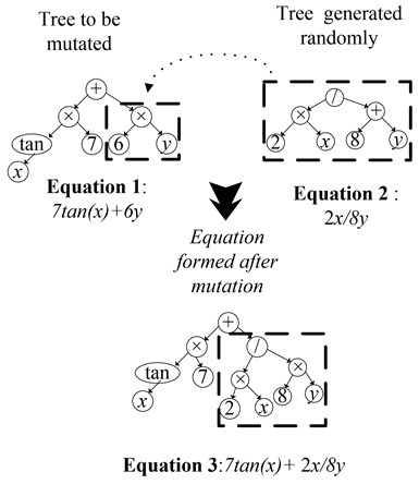
In the second generation, new set of models are developed by applying operators such as crossover, as shown in Fig. 1 and mutation, as shown in Fig. 2, to the models developed in the first stage of generation. In cross-over (Fig. 1), the subtree (part of equation) from both the trees (equations) is selected and swapped. Fig. 1 shows that the subtree is selected from equations A and B and swapped. The swapping is shown by the dotted lines marked in bold in Fig. 1. The cross-over results in formation of the new equations (Equation A1 and B1). In mutation (Fig. 2), a tree (equation) is generated randomly, which replaces the subtree (part of equation) of the selected tree (equation). Fig. 2 shows the mutation mechanism, where the Eq. (3) is formed from the mutation of Eqs. (1) and (2).
These models are then ranked. The least error model then proceeds to the next stage of generation. The error for these models are then evaluated. If it is within the user defined error the model is selected, else the iterative process continues. Once the genetic programming ends, the best model from the population is selected based on minimum error.
Fig. 1Crossover mechanism on models
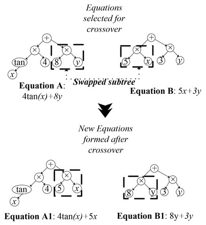
Fig. 2Mutation on models
3. Experimental setup
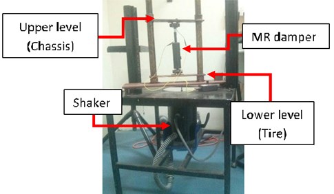
The experimental setup consists of three components: external actuation system, data acquisition system and the controller. The external actuation for the system was fabricated to excite the damper with the help of the electrodynamic shaker. The system was designed to closely depict a quarter car model. The shaker transmits the road disturbances to the lower plate by means of a stringer as seen in the Fig. 3. The lower plate is equivalent to the tire of the vehicle in the quarter car model. The lower plate is coupled with the upper plate with a LORD manufactured MR Damper RD-8040-1 which is a part of the suspension system. The upper plate behaves as the chassis for vehicle. The MR damper is clamped to the upper and lower plates by means of an L clamp.
Fig. 3Experimental setup of MR damper
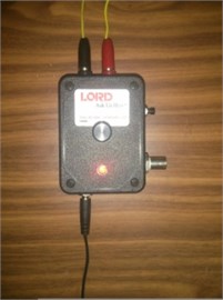
The electro-dynamic shaker (Modal shop Model 2110E) with a load capacity of 489 N (sine-peak) is connected to the linear power amplifier (Crystal Instruments Inc, USA, Model 2050E09) which provides the shaker with the input profile that is given to the system using the Spider 81 data acquisition system (Crystal Instruments Inc., USA) and the associated software (EDM) as shown in Fig. 4. The vibration signals, taken as inputs for genetic programming, are measured using sensors. The signal is measured on the shaker and the lower plate using accelerometers PCB Electronics, Model No. '352C34 LW 155857' of sensitivity 101.3 mV/g and Model No. “352C68 SN 92017” of sensitivity 102.2 mV/g respectively. To measure the force transmitted and the acceleration signals at the upper plate an impedance head, PCB Electronics, Model No. “288D01 SN 3176” is used of sensitivity 98.73 mV/LBF for force and 101.3 mV/g for acceleration. The MR damper is operated using an external power source. The current in the damper is varied using a potentiometer type device called Wonder Box RD-3002-03 manufactured by Lords Corporation, UK as shown in Fig. 5. The current is measured using a multi-meter.
The signal parameters from these sensors are used as inputs for the algorithm and the current that is varied using the potentiometer is used as the output. This current can be directly provided to the control system to create a feedback loop.
Fig. 4Spider 81 and amplifier
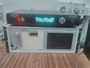
Fig. 5Potentiometer
4. Experimentation
The training set for the genetic programming model is obtained from experimentation using the setup described in section 3. In the experimental setup system, there are 6 factors that are monitored to develop the training set. The experimentation is carried out by varying the frequency and current parameters. The data collected is divided into three sets i.e. 70 % is training set, 15 % is testing set and remaining 15 % is validation. Using this to training set the final model is developed which best fits the data having minimum error. Table 1 provides the configuration of various experiments conducted by varying the parameters.
The input parameters are recorded for 10 seconds of the response. These signatures are as shown in Fig. 6.
Table 1Different test configurations
Sl. No. | Description | Frequency | Steps | Current |
1 | Dwell | 5-7 Hz | 0.1 Hz | 0 A |
2 | Dwell | 5-7 Hz | 0.1 Hz | 0.25 A |
3 | Dwell | 5-7 Hz | 0.1 Hz | 0.50 A |
4 | Dwell | 5-7 Hz | 0.1 Hz | 0.75 A |
5 | Dwell | 5-7 Hz | 0.1 Hz | 1.0 A |
Fig. 6Signatures of acceleration of road profile, lower and upper plate, and signature of force transmitted to upper plate
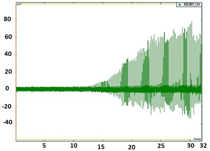
a) Signatures of acceleration of road profile (mm/s2) time
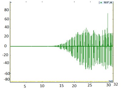
b) Signatures of acceleration of lower plate (mm/s2) time
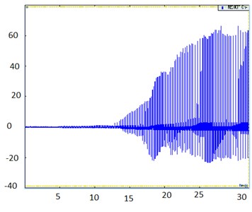
c) Signatures of acceleration of upper plate (mm/s2) time
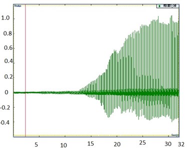
d) Signature of force transmitted () to upper plate
In the first set of tests the current is kept constant and the frequency is increased from 5 Hz to 7 Hz in steps of 0.1 Hz. The data is collected at a sampling rate of 20.48 kHz. In the similar fashion the data set is obtained for all the current values. This data is then consolidated to form the training and testing matrix. There are 4 input parameters taken into consideration in this system:
1) Frequency of excitation;
2) Acceleration of the shaker;
3) Relative acceleration of the upper level (chassis) with respect to the lower level (tire);
4) Force transmitted to chassis.
The current in the damper coils is taken as the output parameter. Using these input-output parameters the genetic algorithm is trained.
5. Results and discussion
We have conducted sufficient preliminary research on the appropriate parameter settings for implementing GP program efficiently on this particular problem. We have performed the trial-and-error procedure to get the appropriate parameter settings. The procedure comprises of the following range of settings. Range of Settings varied from:
1) Population size: 200 to 400;
2) Number of generations: 20 to 100;
3) Maximum tree depth: 5 to 25;
4) Crossover, mutation and reproduction: [0.80-0.90,0.05-0.15,0.05-0.10].
For each of the above-mentioned range, the GP is performed. Based on the minimum RMSE on the training data, we have decided to choose the following settings as given in Table 2. The best model selected from the models generated in the different stages is based on the performance of the model. The algorithm is trained using the parameters shown in the Table 2.
The error for the models obtained in each generation stage is calculated. The model with the least error is then selected. In the results obtained from genetic programming test, three models were formed. The error for all three models are given in Table 3. The model with the least error is chosen from these. This error for this model is shown in red color in Fig. 7. The model equation is:
where, is frequency of excitation, is acceleration of the shaker, is relative acceleration of the upper level (chassis) with respect to the lower level (tire), is force transmitted to chassis.
The parameters for the best model from the population for each generation of the best fitness model is listed in Table 3.
The convergence of the algorithm is based on the selection of the model when the RMSE is minimum. For every run, the best model is selected based on the minimum training RMSE. If there are models with same minimum value of RMSE and different size (number of nodes), the best model with smaller size is selected among them. If there are models with same minimum value of RMSE and same size, then a best model is selected randomly among them. In this way, for the specified number of runs, the best model is selected for each of the run. The final model among these best models is selected again based on the minimum value of RMSE among the runs. In this study, a total of 5 runs are chosen. The best model has training RMSE of 0.11246 and is chosen for finding the equation of output (current).
Fig. 7Error in the best model
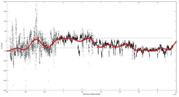
Table 2Parameter for the genetic program
Population size | 300 |
Number of generations | 100 |
Tournament size | 50 |
Max tree depth | 25 |
Max nodes per tree | Infinite |
Using function set | [TIMES MINUS PLUS PLOG TANH TAN SIN COS EXP] |
Number of inputs | 4 |
Max genes | 35 |
Constants range | [–20 20] |
Mutate rate | 1.00E-01 |
Crossover rate | 8.50E-01 |
Reproduction rate | 5.00E-02 |
Table 3Fitness parameters for the best model of each generation
Generation | Training RMSE | Training MAPE | Validation RMSE | Validation MAPE | Test RMSE | Test MAPE | No. of nodes | Depth |
1 | 0.14980 | 65535 | 0.498173 | 55.12169 | 0.77282 | 66.7576 | 139 | 15 |
2 | 0.11188 | 65535 | 0.499335 | 54.0697 | 0.69112 | 65.3761 | 250 | 13 |
3 (Best) | 0.11246 | 65535 | 0.550925 | 56.48313 | 0.72122 | 59.1360 | 247 | 16 |
6. Conclusions
This work is the first of its kind that develops a model to predict the current value to adjust the damper force for the given input parameters, using actual experimental data, in order to maintain the driver acceleration. This model equation can be directly used to design a controller using acceleration, force and driving frequency.
References
-
Liu Wei, et al. Experimental modeling of magneto-rheological damper and PID neural network controller design. 6th International Conference on Natural Computation (ICNC), Vol. 4, 2010.
-
Gandhi Farhan, Inderjit Chopra A time-domain non-linear viscoelastic damper model. Smart Materials and Structures, Vol. 5, Issue 5, 1996, p. 517.
-
Kamath Gopalakrishna M., Norman Werely M. Nonlinear viscoelastic-plastic mechanisms-based model of an electrorheological damper. Journal of Guidance, Control, and Dynamics, Vol. 20, Issue 6, 1997, p. 1125-1132.
-
Snyder Rebecca A., Kamath Gopalakrishna M., Wereley Norman M. Characterization and analysis of magneto-rheological damper behavior due to sinusoidal loading. SPIE’s 7th Annual International Symposium on Smart Structures and Materials, International Society for Optics and Photonics, 2000.
-
Stanway Roger, Sims Neil D., Johnson Andrew R. Modeling and control of a magneto-rheological vibration isolator. SPIE's 7th Annual International Symposium on Smart Structures and Materials, International Society for Optics and Photonics, 2000.
-
Wereley N. M., Pang L., Kamath G. M. Idealized hysteresis modeling of electrorheological and magnetorheological dampers. Journal of Intelligent Material Systems and Structures, Vol. 9, Issue 8, 1998, p. 642-649.
-
Sapiński Bogdan, Jacek Filuś Analysis of parametric models of MR linear damper. Journal of Theoretical and Applied Mechanics, Vol. 41, Issue 2, 2003, p. 215-240.
-
Fujitani Hideo, et al. Dynamic performance evaluations of 200 kN magneto-pheological damper. Technical Note of National Institute for Land and Infrastructure Management, Vol. 41, 2002, p. 349-356.
-
Braz-Cesar Manuel T., Rui Barros Experimental and numerical analysis of MR dampers. 4th International Conference on Computational Methods in Structural Dynamics and Earthquake Engineering (3rd South-East European Conference on Computational Mechanics), 2013.
-
Peng G. R., et al. Modelling and identifying the parameters of a magneto-rheological damper with a force-lag phenomenon. Applied Mathematical Modelling, Vol. 38, Issue 15, 2014, p. 3763-3773.
-
Giuclea Marius, et al. Modelling of magnetorheological damper dynamic behaviour by genetic algorithms based inverse method. Proceedings of the Romanian Academy, Series A, Vol. 5, Issue 1, 2004, p. 5563-5572.
-
Prakash Priyank, Ashok Kumar Pandey Performance of MR damper based on experimental and analytical modelling. Proceedings of the 22nd International Congress of Sound and Vibration, 2015.
Cited by
About this article
Pravin Singru has guided this work from concept of experimental setup to a real setup fabrication, testing and writing the paper. Ayush Raizada has worked on experimental setup fabrication and testing of GP code for modelling. Vishnuvardhan Krishnakumar has been instrumental in taking performing various experiment to generate huge amount of data required for the GP code. Akhil Garg has developed the GP code used in this paper. K. Tai has guided Dr. Akhil to develop the GP code used in this paper.
