Abstract
A novel clustering stabilization diagram combined with self adaptive differential evolution algorithm is proposed to identify the modal parameters of civil engineering structures. Compared with the traditional stabilization diagram, the clustering diagram has drawn more attention because it can distinguish physical and spurious modes due to its automatic performance. In this paper, a self adaptive differential evolution algorithm is proposed to optimize the initial clustering centers so as to improve the clustering stabilization diagram. Moreover, this paper presents a new idea that the modal assurance criterion (MAC) composed of mode shapes is selected as the -axis to replace the model orders or damping ratios in existing stabilization diagrams. The results of a benchmark test of bridge Z24 and the numerical simulation of a continuous beam and a cable-stayed bridge demonstrate the advantages of the proposed approaches and the reliability of detecting the modal parameters.
1. Introduction
Structural health monitoring (SHM) of civil engineering structures is increasingly becoming essential for the occurrence of unavoidable damage during their service life due to environmental, operational and human-induced factors. In SHM, parameter identification is one of the most crucial parts prior to detecting the damage sites and extents, and accurate evaluation of residual life. In the literatures of SHM, ambient excitation-based parameter identification methods combined with modal analysis technique are widely used. Most research efforts had been implemented based on stochastic subspace identification (SSI) method [1-5], wavelet transform method [6], Hilbert transform method [7], and modal analysis in beams [8, 9].
Stabilization diagram used in stochastic subspace identification technique has become a standard tool to estimate modal parameters of civil and mechanical engineering structures in recent decades. The main purpose using the stabilization diagram as a post-processing place for parameter identification is to distinguish physical modes and spurious modes. There are three main causes for spurious modes: First, numerical mathematical spurious modes will arise due to an over-estimation of the system order. Second, noise spurious modes will arise due to physical reasons, e.g. excitation and noise color. Finally, analog or digital filtering of the data also produces numerical spurious poles. The stabilization diagram in combination with the modal similarity index is adopted to effectively indicate spurious modes resulting from noise and model redundancy [10, 11]. Refs. [12, 13] presented the standard deviation of the natural frequencies as horizontal bars in the stabilization diagram. Such a threshold on the standard deviations significantly clears up the diagram, which hence can be used as a stabilization criterion of the identified modes.
Stabilization diagram is simply a plot of different model orders or damping ratios versus the frequencies identified at each of model orders. Generally, the typical stabilization diagram is a graph where the frequency is plotted as the -axis and the model order as the -axis [14-17]. However, the major problem faced by this stabilization diagram is the need for human interaction. In recent years, fuzzy clustering method was introduced as a tool to automatically assess stabilization diagrams figured by damping ratio and frequency. Ref. [18] developed a new technique for the automation of the stability diagrams using the modal phase collinearity and proposed a new cluster validity index which can solve the problem caused by the scale of measurements and which can be directly calculated from non-normalized data. Ref. [19] presented an automatic stabilization diagram based on a hierarchical clustering algorithm to detect the first twelve modes for a long span arch bridge combined with the covariance driven stochastic subspace identification method.
In this paper, a novel clustering stabilization diagram is proposed to detect modal parameter. The modal order or damping ratios are replaced with the MAC composed of mode shapes. As a consequence, the uniqueness of the mode shapes guarantees the accuracy of the proposed approach. Besides, we propose another optimization algorithm, i.e. self adaptive differential evolution (SADE) algorithm to implement the initialization of cluster centers so as to increase the computational efficiency.
This study is organized as follows: In Section 2, the stabilization diagrams are presented including the traditional stabilization diagrams, clustering stabilization diagrams and proposed stabilization diagrams in this study. Section 3 gives the improvements for proposed clustering stabilization diagram to solve the two problems, one is the selection of the column vector in MAC and another is the initialization of the clustering centers. In Sections 4 and 5, the performance of the new stabilization diagram is demonstrated with a benchmark test of bridge Z24 and numerical simulation results from a continuous beam and cable-stayed bridge.
2. Stabilization diagrams
A stabilization diagram is simply a plot figured by model orders and modal parameters identified at each of these orders such as the frequencies, damping ratios and mode shapes. The aim is that physical modes should show up with consistent frequencies, damping ratios and mode shapes at various model orders whereas the spurious ones could be expected to show more erratic behaviour. Due to the difficulty to determine the system order, the actual implementation can be executed by initially choosing a sufficiently high order for the state space model. System identification is performed with every model order. The poles correspond to an order are compared with one order lower system, and they will be plotted in the diagram with different symbols when they meet the following preset criteria as:
where, , and are the frequency, mode shape and damping ratio, respectively. , and are the stability limits with respect to , and , respectively. In this study, the preset stability limits are 1 % for the frequency , 2 % for mode shape and 5 % for the damping ratio . MAC (modal assurance criterion) represents the degree of correlation between two vectors (mode shapes). When the value of MAC equals 1, these vectors are inseparable; when the value of MAC equals 0, the vibration modal vectors are orthogonal and the identified mode shapes for the adjacent model orders are totally different. MAC is defined as follows:
2.1. Traditional stabilization diagram
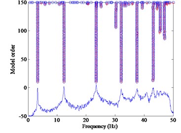
The most common stabilization diagram is called the “traditional stabilization diagram (TSD)” in this study, which is a graph where the frequencies are plotted as the -axis and the model orders as the -axis [14-17]. The TSD shows the poles of a system at different model orders. Physical poles occur at the same frequency at increasing model orders forming a vertical column of poles [11], whereas the spurious numerical poles will not stabilize during this process and can be disregarded more easily [15-20]. The modal parameters are computed from the physical modes at the same order. Fig. 1(a) shows a typical TSD, which is an example of a simple beam bridge excited by white noise in the mispen section (node 6). The finite element model of the beam is discretized into equal length beam elements with 11-node and 10-element, in which the length of each element is 4 meter, the area is 1.075 square meter, the height of the beam is 2 meter and the material density is 7800 kilograms per cubic meter.
It should be noted that the most crucial step of using TSD to identify parameter identification is selecting stable vertical column of poles. In the past, the problem was solved by the interpersonal interaction of expert engineers. However, it is the incorrect determination of the model order and difficulties in discriminating between the physical and the spurious, numerical poles. Thereby, the automation of selecting stable poles became a substantial issue in recent years. The sequential procedure involved in its construction can also interrupt proper grouping of the stable modes once an automatic interpretation algorithm is applied. When a certain stable mode fails to appear in a specific model order, then the grouping procedure might lose track of this mode while investigating the remaining model orders [18]. Moreover, the easy performance is to select the longer vertical column of poles by certain threshold. Pelin Gundes Bakir [11] proposed the ratio of the stable poles to the order to implement the automation of the pole selection process from stabilization diagrams. If this ratio is less than 1/3, then this bin (vertical column of poles) is disregarded.
2.2. Clustering stabilization diagram
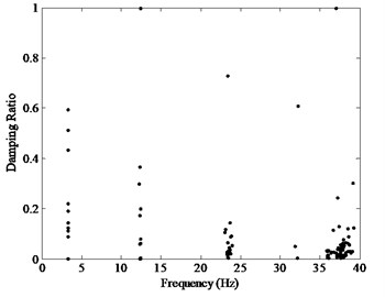
Clustering stabilization diagram (CSD) is a relatively new post-processing tool based on clustering technique, which also shows the poles of a system at different model orders. In present CSD [11, 19, 21], the frequency is plotted on the abscissa and the damping ratio is plotted on the ordinate as shown in Fig. 1(b). After the performance of system identification, the poles satisfied the Eq. (1) will show in the stabilization diagram. The poles from different model orders tend to focus on one point for the physical modes. Instead, the poles involved in spurious modes will disperse and even cannot form a vertical column like the TSD.
The core technique of the CSD is the clustering method. The most widely used clustering method is the fuzzy c-means clustering algorithm (FCM). In the last decades, many researches are focused on improving the standard FCM [20]. However, the clustering methods from FCM are very sensitive to noise because they fail to consider any spatial information. To make FCM more robust to noise, the kernel fuzzy clustering algorithms are proposed [21-24]. In this study, the kernel fuzzy clustering method (KFCM) is used to divide poles into several clusters for parameter identification. The KFCM calculates the objective function through the Euclidean distance and then can improve the Euclidean distance to the different distance measure in the same space.
It is worth mentioning that the major advantage of the CSD superior to the TSD is the automatic performance of the mode selection process [11, 18, 19, 21], even though the clustering process somewhat adds the time of running procedure. The automatic process of CSD depends on the way to compute the distance between the objects concerned [19]. M. Scionti calculated average Euclidian distance of all the members to the cluster prototype and defined a radius of a circle around each cluster. The smaller the circle is, the better the quality of the cluster is. Pelin Gundes proposed a new cluster validity index to compute the inter cluster distance between two modes [11]. If the index between the two modes is less than a certain threshold value, then the two modes represent the same mode and should be included in the same cluster. Otherwise, the clusters represent different modes.
The key problem need to be solved for CSD is the determination of the number of clusters. That can be difficult especially for automated procedures, which may need extensive preprocessing to determine the initial number of clusters. One way to overcome this is a process of similarity based cluster merging [21].
Another problem for CSD is the initialization of the clustering centers. In most cases, it will be the different results for different initial clustering centers. Therefore, a substantial need has recently emerged for the optimization of the initial clustering centers. In Ref. [21], the Genetic Algorithm (GA) has been used to learn cluster centers and to initialize the Fuzzy-C-Means clustering technique membership matrices.
2.3. Proposed stabilization diagram
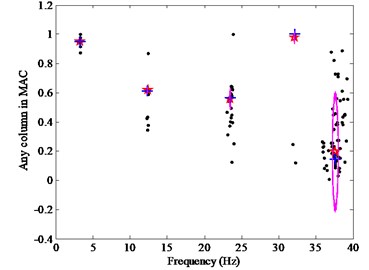
As mentioned previously, the excess amount of user interaction required for picking up the system modes is a drawback of the TSD. In order to overcome these difficulties and automate the selection process, the CSD is adopted to select the stable modes from the large poles of parameters identified at various model orders. However, in the existent clustering stabilization diagrams, damping ratios are adopted as the -axis, whereas they are not very suitable to distinguish modes, owing to the fact that different modes can have the same modal damping ratios and because their estimates present a high scatter [19]. For this reason, we propose a CSD with any column vector in the MAC matrix as the -axis replacing the damping ratios as shown in Fig. 1(c). The consequence should be the poles from different model orders further tend to focus on one point for the physical modes than the CSD with damping ratios vs frequencies. Moreover, the compared circle is presented, whose radius is the average value of the distances from every pole to clustering centers. Thereby, the proposed CSD can achieve automatic identification, because the larger is the circle, the worse the identified result is. In Fig. 1(c), after the number of clusters is determined as five, the objective modes of the first four modes can be judged as the physical modes automatically while the fifth mode corresponding to the larger circle will be removed.
3. Improvements of proposed CSD
Many problems require to be solved for proposed CSD:
• How to select the column vector in MAC matrix as the ordinate of proposed CSD.
• How to initial the clustering centers.
Fig. 1Stabilization diagrams: a) TSD: ○, stable poles with the mode shapes; +, stable poles with the frequency; corrected: (○+), stable poles with both the frequency and mode shape, b) CSD with the frequency vs damping ratios: ●, data poles met Eq. (1), c) Proposed CSD with the frequency versus MAC: ☆, clustering centers; +, nearest poles from the centers; compared circles are plotted with the circles which look like the ellipse or vertical bars due to the different proportion between the X-axis and Y-axis
a)
b)
c)
3.1. Selection of the column vector in MAC
Due to the MAC is a two-dimensional matrix, the one dimensional column vector require to be selected in the process of drawing the clustering view. In order to illustrate how to select the column vector in MAC matrix, the example of the simple beam bridge mentioned above is also used. The columns from 1 to 6 in MAC are used to contrast each other. It should be noted that the selected columns from 1 to 6 can represent the whole performance of MAC due to its symmetry. By using the proposed CSD shown in Fig. 2 combined with the covariance-driven stochastic subspace identification method, the results of the first four mode shapes identified with respect to the column vectors from 1 to 6 in MAC matrix are shown in Fig. 3. Accordingly, the results of the first five frequencies identified are listed in Table 1.
Table 1Results of the first five frequencies with respect to column vectors from 1 to 6 in MAC
Modal order | Column 1 | Column 2 | Column 3 | Column 4 | Column 5 | Column 6 |
1 | 3.272 | 3.273 | 3.273 | 3.273 | 3.272 | 3.272 |
2 | 12.354 | 12.363 | 12.355 | 12.350 | 12.350 | 12.350 |
3 | 23.464 | 23.462 | 23.464 | 23.464 | 23.461 | 23.464 |
4 | 32.103 | 32.102 | 32.103 | 32.103 | 32.101 | 32.103 |
5 | 37.561 | 37.619 | 37.506 | 37.561 | 37.538 | 37.619 |
The results from Fig. 3 and Table 1 show that the selection of different column vector in MAC can almost obtain the same modal parameters. Thereby, we can select the any column vector in MAC as the ordinate in the proposed CSD.
Fig. 2Proposed clustering diagrams with the column vectors from 1 to 6 in MAC
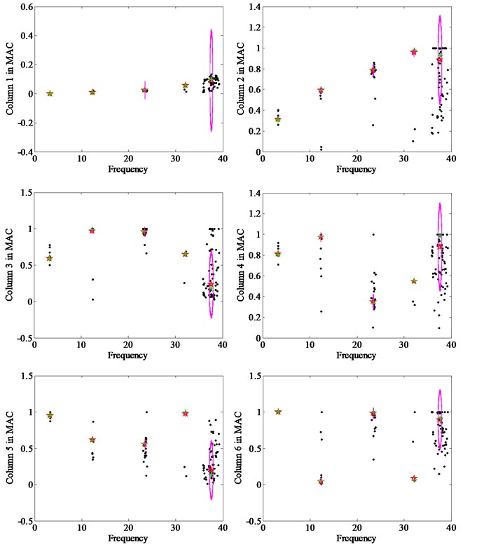
Fig. 3Results of the first four mode shapes with respect to column vectors from 1 to 6 in MAC
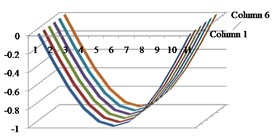
a) Mode 1
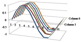
b) Mode 2
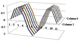
c) Mode 3
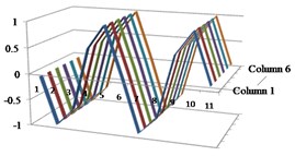
d) Mode 4
3.2. Initialization of the clustering centers
3.2.1. Self-adaptive differential evolution method
The initialization of the clustering centers is a key factor for the identification performance of the clustering diagrams due to the different clustering centers can get the different identification results. If the clustering centers are random, the proposed CSD usually cannot be obtained by once operation of the program. Thereby, a self-adaptive differential evolution method (SADE) [25-27] is proposed to improve the CSD through optimization of the initial clustering centers.
3.2.1.1. Coding
The SADE approach uses real coding, and the individuals are the solutions of the optimization problem. If the data in CSD are divided into clusters with attributes in each cluster, the coding can be expressed as:
3.2.1.2. Mutation
The mutation operation is the biggest difference between the SADE and GA or other algorithms, which is the crucial step in generating the new individual. The middle individual is generated by the linear combination obtained using the following equation:
where , and are three samples selected randomly from the population before the mutation operation. , , , , and is the scaling factor that determines the range of difference vectors and its magnitude scale is from 0 to 1.
Naturally, is disturbed by the random-deviation through the weighted difference between and in the mutation process. Thereby, the compound differences among the individuals become plentiful and the diversity of population is improved.
Above all, is an essential parameter in SADE because it improves the diversity of the population. A small will lead to extensive exploitation in the search space, whereas a large will lead to over exploration and low convergence speed. Therefore, a self-adaptive mutation factor is proposed in this paper, i.e., a small will be adopted to improve the good individuals continually when the value of fitness function is enough large and vice versa.
Moreover, to avoid the premature phenomenon, the value of the scale factor should be large in the initial stage of the algorithm such that the algorithm can maintain the diversities of the individual, search the global optimum value and speed up the convergence speed of the optimal solution. In a later stage of the algorithm, the speed of the scale factor should be decreased, which should make it easy to search for the local optimum value. The dynamic adaptive adjustment equation for the scale factor is shown as follows [28, 29]:
where, is the iteration, and are the maximum and minimum value of the scaling factor, respectively. To maintain the balance between the diversity and the convergence, the value of is [0.5, 1]. is a factor to determine the initial decay rate of the curve, the range of is , in this paper, the value of is 0.001.
3.2.1.3. Cross
The cross operation is undertaken to and to improve the diversity of the population. The new candidate individual is , in which is from 1 to and is from 1 to , and is expressed as:
where is the cross factor determining the probability using the middle individuals to replace the candidate individuals. is the uniformly distributed random number, and is any random integer ensuring that obtains a variable from at least.
3.2.1.4. Selection
In the selection operation, the fitness of the candidate individual is calculated and then compared with the fitness of the individual . The purpose is to determine whether to replace the current individual with the candidate individual:
The selection operation is executed after performing the mutation and cross operations. Meanwhile, the parent individuals compete with the new candidate individuals one by one. Therefore, the new individuals always enter into the next generation with equal opportunities, i.e., the poor individuals are not discriminated in the course of the selection operation.
3.2.2. Initialization
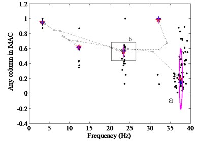
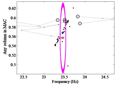
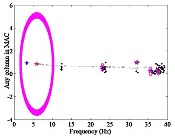
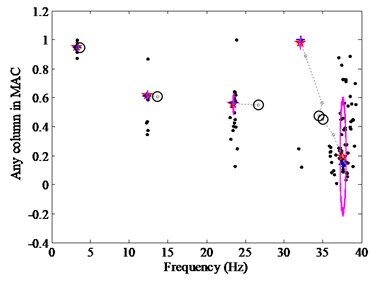
As shown in Figs. 4(a) and (b), the random initialization cannot guarantee the success rate effectively due to the excessive concentration of clustering centers. For example, a typical failed CSD (Fig. 4(c)) will bring out when the program runs many times. In this study, the self-adaptive differential evolution (SADE) is presented as a good tool to initiate the clustering centers. The proposed CSD optimized by the SADE is figured in Fig. 4(d), which can be obtained only by a single operation of the procedure, i.e., there are the same results in the case of multiple times to rerun the procedure. It also can be shown from Figs. 4(a) and (d) that, for the CSD in (a), the clustering centers are centralized so as to the more number of iterations is required to gain the correct results than the CSD in (d), and the clustering centers in (d) are clearly improved.
4. Benchmark test
In the section, the benchmark of bridge Z24 is chosen to verify the proposed method. Some control parameters used in the process of parameter identification for the benchmark test and two examples in Section 5 are same given in Table 2.
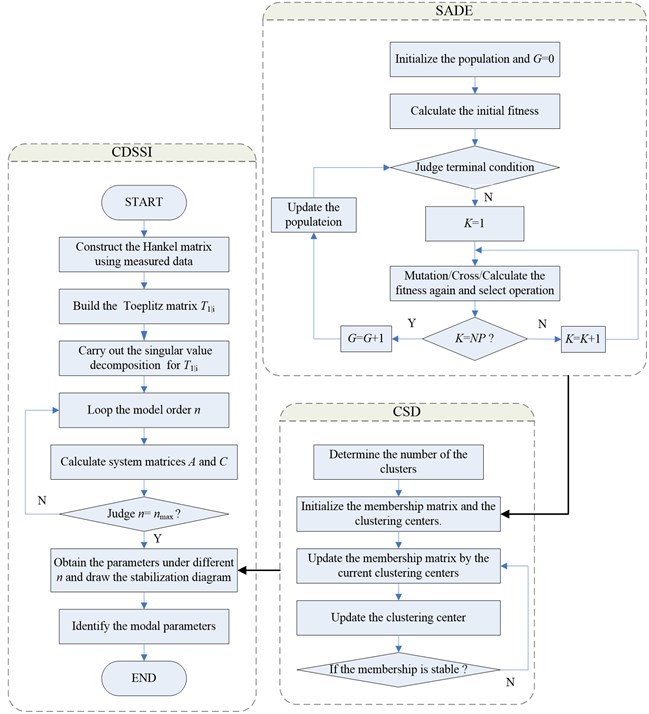
Here, the covariance-driven stochastic subspace identification (CDSSI) method are applied to detect the modal parameter, which has been proved that is one of the most robust and accurate system identification methods for the engineering structures [1-5]. The CDSSI can identify the modal parameters via singular value decomposition of the output covariance matrices based on the stochastic state space model. However, it should be noted that the focus of this paper is on the stabilization diagram combined with the SADE method, rather than the CDSSI method. Therefore, in the benchmark test and the numerical simulations in Section 5, the CDSSI method is applied, but isn’t introduced in detail. The flow chart of the CDSSI with the CSD and SADE is shown in Fig. 5.
Table 2Control parameters used in the process of parameter identification
Parameter | Value |
Model orders | 20-150 |
Limit value of frequency | 1 % |
Limit value of mode shape | 2 % |
Population size | 20 |
Upper boundaries of scaling factor | 1 |
Lower boundaries of scaling factor | 0 |
Cross factor | 0.5 |
Fig. 4Stabilization diagrams for the problem of initialization: a) CSD under the random initialization, b) Enlarged view for the initialized clustering centers in a), c) Failed CSD lusting the second mode, d) CSD optimized by the SADE; ⨀ the initial clustering centers, the running tracks of the clustering centers are plotted using the dash line with small circles
a)
b)
c)
d)
Z24 located in Switzerland is a prestressed concrete bridge with three spans: a midspan of 30 m, two side spans of 14 m each and two cantilevers of 2.7 m (Fig. 6). It should be noted that the intermediate piers are clamed into the main girder, while the end supports with triplets of columns are connected to the girder via hinges. Columns and the end of piers are embedded in the soil. The bridge was artificially damaged in order to study the dynamic response when subjected to progressive damage scenarios. The modal data are identified from ambient vibrations before and after applying each damage scenario. Details about the experimental data can be found in [30].
A simplified FE model is built with ANSYS software, in which 98 beam elements are used for main girder (62 elements), piers and abutment columns (36 elements), 22 spring elements are used to simulate the soil, 6 point mass elements are considered (Fig. 7). Some parameters used in the model are displayed in Table 3.
Table 3FE model parameters of bridge Z24
Parameter | Value | |
Young’s modulus | 37.5 GPa | |
Shear modulus | 16 GPa | |
Poisson’s ratio | 0.2 | |
Soil stiffness | Under the piers, at 14 and 44 m | 180·106 N/m |
210·106 N/m | ||
Under columns, at 0 and 58 m | 100·106 N/m | |
100·106 N/m | ||
At abutments | 180·106 N/m | |
200·106 N/m | ||
Around columns | 100·106 N/m | |
100·106 N/m | ||
Fig. 5Flow chart of the CDSSI using the CSD with the SADE
The FE model is updated by changing the values of Young’s modulus to minimize the difference between the analytical and experimental modal parameters. The initial and updated bending stiffness distribution along the bridge girder is shown in Fig. 8. Consequently, the experimental results are well approximated. The first two bending modes are: 3.89 and 10.30 Hz in experimental modal analysis, 3.73 and 10.25 Hz in [30], 3.89 and 10.56 Hz in [31], and 3.79 and 10.43 Hz in the present CSD (Fig. 9) combined with the CDSSI technique. Regarding the mode shapes, the first and fourth modes, symmetric and non-symmetric respectively are displayed in Fig. 10. Note that the mode shapes results obtained from the present method, Refs. 30 and 31 are all the FE mole results for lack of experimental mode shapes. As can be seen from Fig. 10, the inaccuracy of the first and fourth mode shapes detected by the present CSD, [30] and [31] is small and reasonable.
Fig. 6Highway bridge Z24

Fig. 7FE model of bridge Z24: spring elements (boxes) and point mass elements (black dots)

Fig. 8Initial and updated bending stiffness distribution
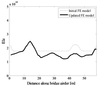
Fig. 9Stabilization diagram using the present CSD
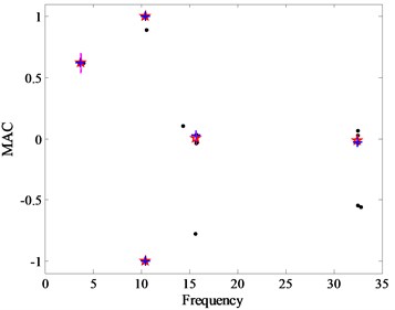
Fig. 10Bending mode shapes from the modal analysis: first and fourth mode
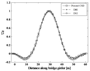
a) Mode 1
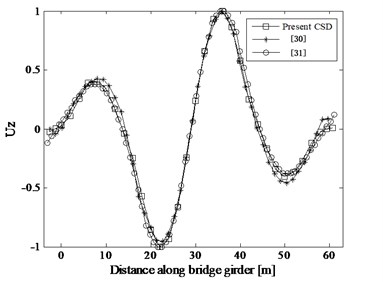
b) Mode 4
5. Numerical simulations
Numerical experiments have been conducted to further test and verify the CSD technique to identify the modal parameters combined with the SADE method. It is expected that the proposed algorithms are more reliable in detecting the structural dynamic parameters. In this paper, we present two numerical examples. They are examples of a continuous beam and a cable-stayed bridge.
5.1. Application in a continuous beam bridge
The effectiveness of the methods proposed in this paper is verified by a three-span continuous beam example in this section. The finite element model is built using the finite element software, in which the entire beam is divided into 30 elements and 31 nodes, as shown in Fig. 11. The physical parameters of the beam are displayed in Table 4.
Table 4Physical parameters of continuous beam
Parameter | Value |
Length of the beam | 60 m |
Depth of section | 1.3 m |
Section area | 0.928 m2 |
Moment of inertia | 0.179 m4 |
Mass density | 2600 kg/m3 |
Elastic modulus | 35 GPa |
The first five modal parameters are calculated by modal analysis for this model to enable a comparison with the identified results. It should be pointed out that only the first five modal parameters are selected as the identified objective even though there are more modes can be detected by the CSD technique combined with the SADE method. White noise excitations of 3.071 seconds are added on nodes 5 and 16, as indicated by the arrows in Fig. 11(a). The vehicle load excitations move from the left end to the right end of the continuous beam within 2.401 seconds shown in Fig. 11(b).
Fig. 11Finite element model with different excitations

a) Nodes 5 and 16 excited by white noise

b) All nodes excited by a moving load
5.1.1. Continuous beam excited by white noise
The white noise excitation can be used to simulate the ambient excitation. In this study, the sampling frequency is 1000 Hz, i.e., there are 3071 strain data to be extracted on each node during sampling time; at the same time, 307×131 95201 strain data are prepared as the input data of the CDSSI.
5.1.1.1. Traditional stabilization diagram
The TSD can be regarded as a good way to identify the modal parameters, although it is not so automated. To enable a comparison with the CSD, the TSD is established as shown in Fig. 12(a).
As a result, the TSD based on the CDSSI can precisely identify the first five frequencies and mode shapes. Moreover, the first five poles can be identified as the physical modes because they are sufficiently long. However, the identification process requires the judgment of experts, which is the only flaw of the TSD.
5.1.1.2. Clustering stabilization diagram
The CSD based on the KFCM and SADE is applied to the analysis of this continuous beam, in which the frequency is the abscissa and the sixteenth column value in MAC matrix is the ordinate. After the determination of the number of cluster is , the CSD combined with SADE is presented in Fig. 12(b). As shown in Fig. 12(b), after the twelfth mode is determined, which corresponds to the larger circle being removed, the objective modes of the first five orders can be judged as the physical modes automatically. In detail, the radii of all the compared circles are listed in Table 5.
Note that while the above analysis has focused on white noise excitation, the reliability of this proposed method still should be examined for the case of more complex natural excitation with ambient noise. As a result, the following work was performed for a continuous beam excited by a vehicle load.
Table 5Radius results of all compared circles in Fig. 5(b)
Clustering number | 1 | 2 | 3 | 4 | 5 | 6 | 7 | 8 | 9 | 10 | 11 | 12 |
Radius | 0.0006 | 0.0002 | 0.0055 | 0.0000 | 0.0008 | 0.0203 | 0.0000 | 0.0001 | 0.0147 | 0.0186 | 0.0141 | 0.2865 |
Fig. 12Stabilization diagrams: a) TSD, b) CSD optimized by SADE. The criteria are 1 % for frequencies, 5 % for damping ratios, 2 % for mode shape vectors (MAC)
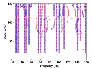
a)
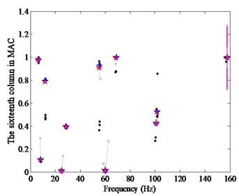
b)
5.1.2. Continuous beam excited by a moving load
The vehicle load excitations are used here because they are closer to the actual situation of the natural ambient. However, the ambient noises are the main factors that affect the accuracy of the identified results in a practical project. The dynamic response data with noise can be calculated by the following equation:
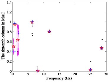
where is the measured value, is the noise level and is the Gaussian random number, the mean of which is zero and the variance is one. Two noise levels are considered, with and . The results of the CSD with the SADE are shown in Fig. 13 when the all of the data are divided into eight clusters.
Fig. 13CSD with different noise levels
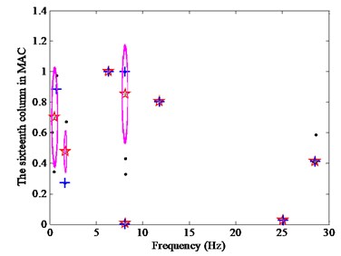
a) 5 %
b) 10 %
5.1.3. Results of the parameter identification
The modal parameters of the continuous beam can be extracted by the poles in the TSD (Fig. 12(a)) and the nearest data points from the clustering centers in the CSD with the SADE (Figs. 12(b) and 13). For the convenience of the comparative analysis, a summary frequency results calculated by the finite element model, identified as TSD and CSD, with the different excitations and noise levels are listed in Table 6. The error of the modal frequencies in TSD and CSD under the white noise excitation is less than 2.22 %, while the maximum value of the frequency error is only 0.28 % when the beam is excited by the moving load. Correspondingly, the first five strain mode shapes are shown in Fig. 14. When all of these results are considered together, we can conclude that the first five frequencies and mode shapes of the continuous beam can be identified accurately; of course, the CSD with SADE is better than TSD in terms of the performance of the automated process. In addition, the CSD can still detect the modal parameters precisely when the different noises are added into the measured data, which means the novel CSD using the KFCM and the SADE proposed in this study has the higher interference ability, accuracy and reliability performance.
Fig. 14Strain mode shapes, including the model, TSD, and CSD with different excitations and noise levels
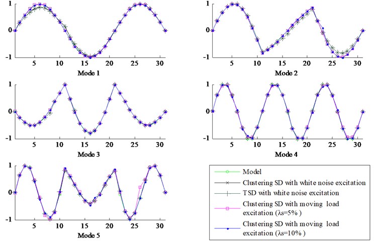
Table 6Comparative results of frequency with respect to different SD and model
Modal order | Model frequency (Hz) | TSD | CSD (White noise excitation) | CSD (Moving load excitation) | |||||
Frequency (Hz) | Error (%) | Frequency (Hz) | Error (%) | Frequency (Hz) ( 5 %) | Error (%) | Frequency (Hz) ( 10 %) | Error (%) | ||
1 | 6.31 | 6.38 | 1.11 | 6.37 | 0.95 | 6.31 | 0 | 6.31 | 0 |
2 | 8.09 | 8.27 | 2.22 | 8.27 | 2.22 | 8.09 | 0 | 8.09 | 0 |
3 | 11.81 | 11.86 | 0.42 | 11.86 | 0.42 | 11.8 | –0.08 | 11.8 | –0.08 |
4 | 25.08 | 25 | –0.32 | 25 | –0.32 | 25.03 | –0.20 | 25.02 | –0.24 |
5 | 28.57 | 28.54 | –0.11 | 28.54 | –0.11 | 28.5 | –0.25 | 28.49 | –0.28 |
5.2. Application in a cable-stayed bridge
5.2.1. Parameter identification using proposed CSD and SADE
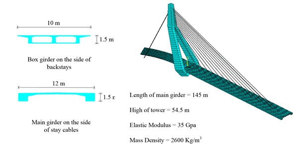
The second numerical example considered is a cable-stayed bridge with backstays shown in Fig. 15. The finite element model is built by the finite element software in which the main girder, tower and cable are simulated by the elements of beam189, beam44 and link10, respectively.
The girder is excited using vertical seismic waves from Tianjing that the length of time is 19.12 seconds and sampling rate is 100 Hz for the vertical displacement. The response of displacement time history is computed using finite element analysis which is used for the input data of CDSSI combined with CSD and SADE. The number of clustering is selected as 15. The results of the stabilization diagrams are shown in Fig. 16 when the ordinates of the diagrams are chosen as the eighth column in MAC matrix, i.e. the data of the direction displacement are obtained from the crossed node between the eighth cable and main girder.
Fig. 15Cable-stayed bridge
5.2.2. Results of the parameter identification
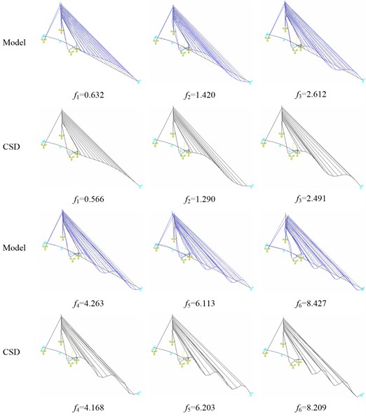
The modal parameters of the cable-stayed bridge can be observed automatically from the stabilization diagrams (Fig. 16). Fig. 17 shows the results of the first six vertical mode shapes, which present a contrastive analysis between the finite element model and CSD proposed in this paper. Accordingly, the results for the frequencies are also shown in the figure. However, the errors of the first two mode shapes and frequencies are relatively larger than the last four ones. Speaking with numbers corresponding to the results of the finite element model, the errors of the first two frequencies identified are up to 10.44 % and 9.15 %, respectively, but the largest error in the last four frequencies is only 4.63 %.
Fig. 16Stabilization diagram of CSD with SADE for UY displacement
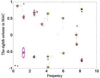
Fig. 17The first six vertical mode shapes and frequencies
6. Conclusions
An improved clustering stabilization diagram combined with self-adaptive differential evolution is proposed for parameter identification in this paper. The TSD and the proposed CSD are all the powerful tool to remove the spurious modes from the numerous modes. The proposed CSD plotted by the frequency and MAC is more reliable than the other stabilization diagram consisting of the frequency and damping ratio and better than the TSD in terms of its automatic performance. In particular, the presented SADE algorithm played a crucial role in improving the success rate of the CSD to identify the parameters by optimizing the initial clustering centers. Benchmark test of bridge Z24 and numerical simulations of a continuous beam under different excitations and a cable-stayed bridge verified that the proposed method is effective and reliable in parameter identification in civil engineering structures. Future studies will focus on the application of the proposed method in more complex bridges with measured data.
References
-
Alicioglu Bilge, LusHilmi Ambient vibration analysis with subspace methods and automated mode selection: case studies. Journal of Structural Engineering, Vol. 134, Issue 6, 2008, p. 1016-1029.
-
Cho Soojin, Park Jong-Woong, SimSung-Han Decentralized system identification using stochastic subspace identification for wireless sensor networks. Sensors, Vol. 15, 2015, p. 8131-8145.
-
Dong Xiaofeng, Lian Jijian, Yang Min, Wang Haijun Operational modal identification of offshore wind turbine structure based on modified stochastic subspace identification method considering harmonic interference. Journal of Renewable and Sustainable Energy, Vol. 6, 2014, p. 033128.
-
Wang L. X., Di S. K. Modal parameter identification of concrete filled steel tube arch bridge based on stochastic subspace method. Advanced Materials Research, Vols. 919-921, 2014, p. 325-328.
-
Al Gahtani O., El Gebeily M., Khulief Y. Output-only identification of system parameters from noisy measurements by multiwavelet denoising. Advances in Mechanical Engineering, Vol. 6, 2014, p. 218328.
-
Sarparast H., Ashory M. R., Hajiazizi M., Afzali M., Khatibi M. M. Estimation of modal parameters for structurally damped systems using wavelet transform. European Journal of Mechanics A/Solids, Vol. 47, 2014, p. 82-91.
-
Yang Kai, Yu Kaiping, Li Qiaofeng Modal parameter extraction based on Hilbert transform and complex independent component analysis with reference. Mechanical Systems and Signal Processing, Vol. 40, 2013, p. 257-268.
-
Yayli Mustafa Özgür On the axial vibration of carbon nanotubes with different boundary conditions. Micro and Nano Letters, Vol. 9, Issue 11, 2014, p. 807-811.
-
CercevikYayli Axial vibration analysis of cracked nanorods with arbitrary boundary conditions. Journal of Vibroengineering, Vol. 17, Issue 6, 2015, p. 2907‑2921.
-
Zhang Guowen, Tang Baoping, TangGuangwu An improved stochastic subspace identification for operational modal analysis. Measurement, Vol. 45, 2012, p. 1246-1256.
-
BakirPelin Gundes Automation of the stabilization diagrams for subspace based system identification. Expert Systems with Applications, Vol. 38, 2011, p. 14390-14397.
-
Döhler Michael, MevelLaurent Efficient multi-order uncertainty computation for stochastic subspace identification. Mechanical Systems and Signal Processing, Vol. 38, 2013, p. 346-366.
-
Döhler Michael, MevelLaurent Fast multi-order computation of system matrices in subspace-based system identification. Control Engineering Practice, Vol. 20, 2012, p. 882-894.
-
Mrabet E., Abdelghani M., Benkahla N. A new criterion for the stabilization diagram used with stochastic subspace identification methods: an application to an aircraft skeleton. Shock and Vibration, Vol. 2014, Issue 2014, p. 2014-409298.
-
Javier Cara F., Jesús Juan, Enrique Alarcón, Edwin Reynders, Guido De Roeck Modal contribution and state space order selection in operational modal analysis. Mechanical Systems and Signal Processing, Vol. 38, 2013, p. 276-298.
-
Gert De Sitter, Christof Devriendt, Patrick Guillaume Transmissibility-based operational modal analysis: Enhanced stabilisation diagrams. Shock and Vibration, Vol. 19, 2012, p. 1085-1097.
-
Tondrea Gilles, DeraemaekerArnaud Numerical and experimental analysis of uncertainty on modal parameters estimated with the stochastic subspace method. Journal of Sound and Vibration, Vol. 333, 2014, p. 4376-4401.
-
Alıcıoğlu B., Luş H. Ambient vibration analysis with subspace methods and automated mode selection: case studies. Journal of Structural Engineering, Vol. 134, 2008, p. 1016-1029.
-
Magalhães F., Cunha Á., Caetano E. Online automatic identification of the modal parameters of a long span arch bridge. Mechanical Systems and Signal Processing, Vol. 23, 2009, p. 316-329.
-
Peeters B. Comparative study of modal analysis techniques for bridge dynamic characteristics. Mechanical Systems and Signal Processing, Vol. 17, Issue 5, 2003, p. 965-988.
-
Scionti M., Lanslots J. P. Stabilisation diagrams: Pole identification using fuzzy clustering techniques. Advances in Engineering Software, Vol. 36, 2005, p. 768-779.
-
Wu Z., Gao X., Xie W., Yu J. Kernel method-based fuzzy clustering algorithm. Journal of Systems Engineering and Electronics, Vol. 16, 2005, p. 160-166.
-
Graves Daniel, Pedrycz Witold Kernel-based fuzzy clustering and fuzzy clustering: a comparative experimental study. Fuzzy Sets and Systems, Vol. 161, 2010, p. 522-543.
-
Cong Zhang, Shan Zeng, Hui Zhang Electrocardiography classification based on revised locally linear embedding algorithm and kernel-based fuzzy C-means clustering. Journal of Medical Imaging and Health Informatics, Vol. 4, 2014, p. 916-921.
-
Price K. V., Storn R. M., Lampinen J. A. Differential Evolution: a Practical Approach to Global Optimization. Springer, 2005.
-
Farzan Rashidi, Ebrahim Abiri, Taher Niknam On-line parameter identification of power plant characteristics based on phasor measurement unit recorded data using differential evolution and bat inspired algorithm. Science Measurement and Technology, IET Science Measurement and Technology, Vol. 9, 2015, p. 376-392.
-
Kovačević Darko, Mladenović Nenad, Petrović Bratislav, Milošević Pavle DE-VNS: self-adaptive differential evolution with crossover neighborhood search for continuous global optimization. Computers and Operations Research, Vol. 52, 2014, p. 157-169.
-
Deng Wu, Yang Xinhua, Zou Li, Wang Meng, Liu Yaqing, Li Yuanyuan An improved self-adaptive differential evolution algorithm and its application. Chemometrics and Intelligent Laboratory Systems, Vol. 128, 2013, p. 66-76.
-
Wu L. H., Wang Y. N. Self-adapting control parameters modified differential evolution for trajectory planning manipulator. Control Theory Application, Vol. 5, Issue 4, 2007, p. 365-373.
-
Teughels A., De Roeck G. Structural damage identification of the highway bridge Z24 by FE model updating. Journal of Sound and Vibration, Vol. 278, 2004, p. 589-610.
-
Masciottaetal M.-G. A spectrum-driven damage identification technique: application and validation through the numerical simulation of the Z24 Bridge. Mechanical Systems and Signal Processing, Vol. 70, Issue 71, 2016, p. 578-600.
Cited by
About this article
This work was supported by the “985 Project” of Jilin University, the National High Technology Research and Development Program of China and the National Natural Science Foundation of China (Nos. 51378236). The financial support is gratefully acknowledged.
