Abstract
In this paper four non-parametric and five parametric signal processing techniques are reviewed and their performances are compared through application to a sample exponentially damped synthetic signal with closely-spaced frequencies representing the ambient response of structures. The non-parametric methods are Fourier transform, periodogram estimate of power spectral density, wavelet transform, and empirical mode decomposition with Hilbert spectral analysis (Hilbert-Huang transform). The parametric methods are pseudospectrum estimate using the multiple signal categorization (MUSIC), empirical wavelet transform, approximate Prony method, matrix pencil method, and the estimation of signal parameters by rotational invariance technique (ESPRIT) method. The performances of different methods are studied statistically using the Monte Carlo simulation and the results are presented in terms of average errors of multiple sample analyses.
1. Introduction
Vibration-based structural health monitoring (SHM) has become increasingly popular in recent years as a general and global method to detect possible damage scenarios [1-4] unlike optical observations that can detect only superficial and localized damage [5, 6] or nondestructive testing methods such as radiography or x-ray [7].
The main step in any SHM approach is the processing of collected response signals (Sun et al., 2015). In this stage, signals are analyzed to extract specific features such as modal parameters or directly create a model that fits the data as in system identification (SI). Similar to parametric (white or grey box) and non-parametric (black box) system identification categorization based on the prior knowledge of the model, signal processing methods are divided into parametric and nonparametric methods based on the knowledge of the signal source [8, 9]. Parametric signal processing methods exploit the a priori knowledge to obtain physical features or structural parameters such as natural frequencies or damping ratios [10]. When the number of the degrees-of-freedom (DOFs) of the signal source model is known, then the number of constituent modes in the signal is also known and expected to be equal to the same number. An example is free vibration response of a multi-DOF structure described in the following section.
Recorded vibration signals, however, are often noisy owing to data recording equipment and collection processes [11, 12]. Using filters reduces the noise content and improves the performance of SI approaches. Nonparametric methods are used when no prior knowledge about signal is available such as traffic flow, speed, or occupancy signals [13-21]. Another example is the electrocardiogram (ECG) signal obtained from the heart [22-24]. A third example is the electroencephalogram (EEG) signal obtained from the brain [25-30].
In SHM collected signals can be used two different ways, either to directly create a model such as auto regressive (AR), state space, or artificial neural network models [31] with no signal processing, or to extract specific features that are sensitive to damage and can be used for damage detection using signal processing techniques. The second approach and the use of signal processing methods to extract features, specifically natural frequencies and damping coefficients, is the focus of this paper. These features can further be used directly to detect damages through classification algorithms or used to create an updated model of the structure as in the finite element model updating approach.
In the next section, a sample synthetic signal including four damped sinusoids where two have relatively closely-spaced frequencies is described to be used for comparative analysis of existing signal processing methods. Next, four non-parametric signal processing methods are applied to the synthetic signal and their shortcomings are pointed out. This is followed by application of five parametric signal processing techniques. The performances of different methods are studied statistically using the Monte Carlo simulation and the results are presented in terms of average errors of multiple sample analyses.
2. Sample signal
In dynamic analysis of discrete (lumped mass) structures, the equation of motion for an m DOF system is a second order differential equation in the form [32]:
where M is the m×m mass matrix, C is the m×m damping coefficient matrix, K is the m×m stiffness matrix, x is the displacement vector and f is the time-dependent loading vector. Considering f to be a null vector, the general solution for a free vibration response is in the form:
=∑mi=1φ'jie-ξiωitcos(ωdit+θ'i),
where i refers to the mode number, j refers to DOF, φji is the amplitude vector of the ith mode shape at DOF j, ξi=Ci/2Miωi is the damping ratio of the ith mode, ωdi=ωi√1-ξ2i is the damped natural frequency of the ith mode, ωi is the ith undamped natural frequency, and θ is the phase angle for the ith mode. Eq. (2) is in the form of an exponentially damped harmonic signal. It can be seen that the related speed and acceleration signals are also sums of damped sinusoids though with different amplitudes and phase angles. Therefore, during free vibration of a multi-DOF structure, a sensor (displacement, velocity, or acceleration) placed on any of the DOFs is expected to record a signal including multiple damped sinusoids.
Inspired by Eq. (2), the sample signal used in this research for testing various signal processing algorithms is obtained by a superposition of four different damped sinusoid waves with frequencies of 0.3, 0.5, 1 and 1.5 Hz, the first two chosen intentionally to be close, plus white noise (ϵ) with a signal to noise ratio (SNR) of 5 dB. The synthetic signal is sampled at 0.05 seconds for a length of 12 seconds. The resulting equation for the signal shown in Fig. 1 is:
+e-0.7tcos(1.5×2π×t)+ϵ.
Fig. 1Synthetic signal used in this research Eq. (3)
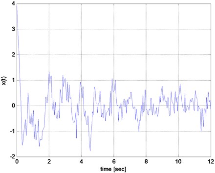
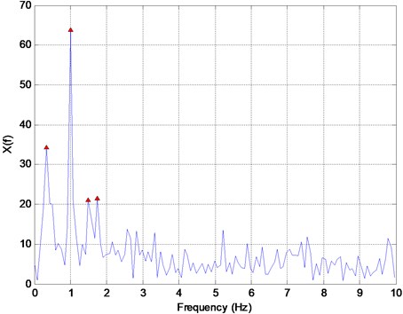
Fig. 2Fourier transform of the signal shown in Fig. 1. The estimated frequencies (the first four peak noted by triangles) are 0.33, 0.99, 1.49, and 1.74
3. Nonparametric signal processing methods
3.1. Fourier transform
Fourier transform (FT) is the most widely-used method to represent the frequency domain of a time series signal. Assuming that the signal x(t) has finite energy, that is:
the discrete Fourier transform (DFT) is defined as:
where N is the length of signal (number of sampling points), f=k/N is the frequency in cycles per sample, ω=2πk/N is the circular frequency in radians/sample, and i is the sample index (e.g. time increment). The Fourier transform of the synthetic signal (Fig. 1) is shown in Fig. 2. The estimated frequencies (the first four peaks noted by triangles in Fig. 2) are 0.33, 0.99, 1.49, and 1.74 Hz. Table 1 presents the estimated values of frequency and damping exponents for the methods studied in this research. In the results of DFT method, the first two damped frequencies are mixed as one peak at around 0.33 Hz. This is a drawback of the FT method that cannot extract all the frequencies accurately when the signal is a) noisy, b) has closely-spaced frequencies, or c) is non-stationary. Moreover, the 4th peak with a value of 1.74 Hz, is a spurious solution, another drawback of the FT. Furthermore, FT provides no information about the damping values.
3.2. Periodogram estimate of power spectral density (PSD)
The power spectral density (PSD), a measure suitable for analysis of stationary signals, is defined as the Fourier transform of the autocorrelation sequence of the sample signal. It is often estimated by a periodogram with a rectangular window, defined by magnitude squared of DFT coefficients as follows:
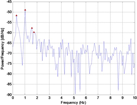
where Ts is the sampling time interval and f is frequency in Hz, 0<f≤1/2Ts due to Nyquist Sampling theorem. The PSD of the sample signal is shown in Fig. 3. Table 1 presents the estimated values of the four frequencies. Similar to DFT, it represents two frequencies accurately but the first two closely-spaced modes are mixed together and indistinguishable. The 4th frequency at 1.73 is a spurious solution. As such, PSD also suffers from both problems of mixing closely-spaced frequencies and generating spurious solutions. Further, PSD shows noisy characteristics with many spurious peaks.
Fig. 3Power spectral density (PSD) of the signal in Fig. 1 with the peak frequency values of 0.31, 1.02, 1.57, and 1.73
3.3. Wavelet transform
In the past two decades wavelet transform has been used extensively as a time-frequency signal processing method in a variety of applications such as seismology [33]; structural and mechanical vibrations [34], vibration control [35], system identification [36], power engineering [37], computational neuroscience [38, 39], traffic engineering [40-43] and SHM [44]. In contrast to FT where sinusoidal functions are used, in continuous wavelet transform a base function with localized energy is used to approximate the signal. The signal is decomposed into different variations of the base function and presented as an integral of scaled and dilated wavelets. The coefficients are found from the following transformation represented by a two-dimensional matrix W:
where a and b are the scale and the dilation parameters, and Ψ is the base wavelet function, called mother wavelet.
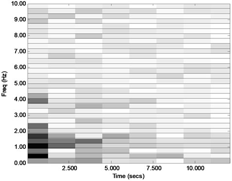
In discrete wavelet transform (DWT), two quadrature mirror filters, one low pass and one high pass are used in the first level of transformation. The results from high pass and low pass filters are called detail and approximation coefficients, respectively. Since each output contains half of the frequency range, they are subsampled by 2. As such, the time resolution will be only half of the original signal. This process is repeated to calculate all coefficients representing higher frequency resolutions. To improve the accuracy, wavelet packet transform (WPT) [45, 46] has been proposed where both approximation and detail signals are decomposed. Fig. 4 shows the values of the calculated WPT coefficients of the synthetic signal shown in Fig. 1 in time and frequency domains using the widely-used Daubechies wavelet of the 1st order. This figure is known as a scalogram. The estimated values of the four frequencies presented in Table 1 indicate a concentration of the frequency content at about 0.5, 1, and 1.5 Hz noted by dark rectangles and the dissipation in time, as expected, noted by lightening of the rectangles. However, the time-resolution is coarse and the closely-spaced frequencies at 0.3 and 0.5 Hz are mixed together as one and indistinguishable. The result may improve by choosing a higher frequency resolution but at the cost of a lower time resolution. Also, the wavelet type selected has some bearing on the accuracy which makes it problem-dependent or a subjective decision making process. WT and WPT are indeed effective for detecting sudden changes in a signal but less effective for extracting the contents of smoothly changing or exponentially decaying signals.
Fig. 4Scalogram of the synthetic signal shown in Fig. 1 using the wavelet packet decomposition
3.4. Empirical mode decomposition (EMD) with Hilbert spectral analysis (Hilbert-Huang transform)
The empirical mode decomposition (EMD) method is a time domain signal processing approach that decomposes a signal into Intrinsic Mode Functions (IMFs). It is used as the first step of Hilbert-Huang transform (HHT) where Hilbert spectral analysis is performed on the extracted IMFs to obtain the instantaneous frequency contents of the data [47]. HHT was proposed mainly for analysis of non-stationary nonlinear signals. Any given time domain signal x(t) is decomposed into n-1 oscillating and one non-oscillating IMFs:
The method yields all modes with no prior information about the number of signal components (n) which makes it attractive for non-parametric signal processing. First, all local maxima and minima of the original signal are detected. Then, two envelopes including all maxima and minima are calculated as a function of time, ¯x(t) and x_(t), respectively. Then, the mean of these two time functions is deducted from the original signal:
This process is repeated for the residual x1(t) signal until the mean vector approaches a null vector within a given tolerance. The last residual sequence is the first extracted IMF, IMF1(t), of the signal which usually includes the highest frequency content. This process is repeated for x(t)-∑iIMFi(t) until the last remainder has only one maximum or minimum.
Next, an imaginary signal introduced by [48] as the analytic signal is created as follows:
where y(t) is the Hilbert transform of the signal, x(t):
Hilbert transform of a signal is in fact the convolution integral of the signal and 1/πt. The analytic signal as a complex signal can be expressed in terms of the magnitude and the phase angle, θ(t), where the instantaneous frequency is the time derivative of the phase angle:
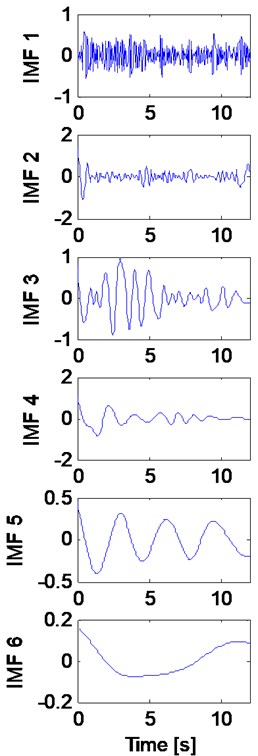
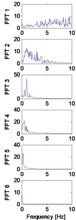
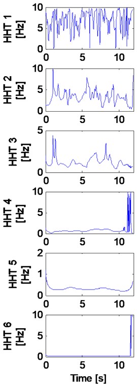
Fig. 5(a) and Fig. 5(b) show the extracted IMFs of the synthetic signal (Fig. 1) using the EMD approach and the corresponding FFTs, respectively. The first IMF contains the fastest oscillation content of the data and the last IMF is in fact not an oscillatory signal at all. FFTs show the frequency content moves from the high frequency range to the low-frequency range as the number of IMF increases. This means the lower-level IMFs represent the high-frequency content and the higher-level IMFs represent the low-frequency content. Fig. 5(c) presents the Hilbert spectra of extracted IMFs. In the EMD method, each IMF is ideally expected to be a separate/unique exponentially decaying sinusoid with but this separation may not be realized in real-life signals such as those obtained in SHM. For example, in Fig. 5(c), modes are mixed. If the modes were not mixed the instantaneous frequency plot of the HHT would indicate an almost constant value for each IMF (it is mostly constant for IMFs 4, 5, and 6 but not the others). Another shortcoming of HHT is that it generates spurious modes. For example, the original uncontaminated synthetic signal used in this research has four intrinsic frequencies but the HHT produces 5 oscillatory IMFs.
Table 1Comparison of modal parameter estimation using sifferent parametric and non-parametric signal processing methods ***
FT | PSD | EWT * | MUSIC | ESPRIT | Matrix Pencil | Prony | Original value | ||
1st frequency | Value | 0.33 | 0.31 | 0.05** | 0.29 | 0.32 | 0.33 | 0.20 | 0.30 |
Error (%) | 10.0 | 3.3 | 82.3 | 3.3 | 6.0 | 10.0 | 32.7 | – | |
1st damping | Value | – | – | – | – | – | 0.37 | 0.28 | 0.30 |
Error (%) | – | – | – | – | – | 23.3 | 6.7 | – | |
2nd frequency | Value | 1.74** | 1.73** | 0.61 | 9.47** | 2.42** | 2.51** | 0.55 | 0.50 |
Error (%) | 248.0 | 246.0 | 22.0 | 1794.0 | 384.8 | 401.4 | 9.2 | – | |
2nd damping | Value | – | – | – | – | – | 0.29 | 1.06 | 1.00 |
Error (%) | – | – | – | – | – | 71.3 | 6.0 | – | |
3rd frequency | Value | 0.99 | 1.02 | 1.00 | 0.99 | 1.00 | 1.00 | 1.00 | 1.00 |
Error (%) | 1.0 | 2.0 | 0.1 | 1.0 | 0.2 | 0.2 | 0.1 | – | |
3rd damping | Value | – | – | – | – | – | 0.14 | 0.16 | 0.15 |
Error (%) | – | – | – | – | – | 4.1 | 6.0 | – | |
4th frequency | Value | 1.49 | 1.57 | 1.45 | 1.57 | 1.46 | 1.46 | 9.82** | 1.5 |
Error (%) | 0.7 | 4.7 | 3.3 | 4.7 | 2.8 | 2.7 | 554.3 | – | |
4th damping | Value | – | – | – | – | – | 0.97 | 1.61 | 0.7 |
Error (%) | – | – | – | – | – | 39.0 | 130.3 | – | |
Avg. Err | 64.9 | 64.0 | 26.7 | 450.7 | 98.5 | 70.2 | 92.6 | ||
* Frequencies are estimated from each extracted sub signal ** Spurious frequency *** Only the methods providing parameter values are considered in the table. | |||||||||
4. Parametric signal processing methods
4.1. Pseudospectrum estimate using Music
Most parametric signal processing methods estimate the signal as a sum of a certain number of complex exponentials. In the methods that represent a real valued signal by a sum of complex exponentials, such as free vibration response of a d-DOF system, 2×d complex exponential components must be found to cover all corresponding dynamics of the system. For example, for any given sinusoidal signal, two complex conjugate exponentials are found whose summation forms the sinusoidal signal. If there is a complex eigenvalue in a real-valued matrix, its conjugate is also an eigenvalue of the matrix. As such, the number of signal components is twice the number of DOFs.
Knowing the number of the signal components, D=2d, a priori, the multiple signal classification (MUSIC) approach uses estimates of the eigenvectors of a correlation matrix associated with the data vector to calculate a corresponding pseudospectrum [49, 50]. For a given signal of length N (a column vector with N rows) presented as vector x, it is assumed that the signal is defined as the sum of M complex exponential sequences plus noise:
where αk, ωk, φk are the amplitude, frequency, and phase angle of the kth complex exponential sequence and u is the zero mean white noise signal of length N. If X is a rectangular Toeplitz matrix of x, the covariance matrix of size N×N is defined and decomposed as [51, 52]:
where E is the expectation operator used for considering different observations of the signal, A is the eigenvector matrix of size N×D, P is an D×D diagonal matrix of the estimates of amplitudes squared, α2k, I is the identity matrix of size N×N, σ2 is the noise variance, and AH is the Hermitian or conjugate transpose of A matrix. Then, x is estimated as:
where vector p includes estimates of αk with length M such that P=E(ppH). The eigenvectors corresponding to M largest eigenvalues of Rx span the signal subspace and the eigenvectors corresponding to the remaining eigenvalues of size J=N-D form the noise subspace.
Fig. 5a) Extracted IMFs using EMD method, b) corresponding FFT, and c) Hilbert transforms
a)
b)
c)
The pseudospectrum values are in fact the inverse of the Euclidian distances of all the sinusoidal sequences in the frequency range to the noise space formed by J eigenvectors. The peaks in the pseudospectrum plot versus frequency is expected to reveal the frequency content of the signal. The equation for pseudospectrum as a function of frequency f value is:
where G is the N×J matrix of noise eigenvectors, and b(f) is the vector of terms in a geometric progression of exponentials with complex exponent if:
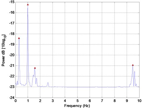
To improve the time resolution in this research the pseudospectrum calculation is done for shorter lengths of x by windowing the main signal with overlapping windows. This way the dimension N is replaced by the window length in Eqs. (10)-(14). Fig. 6 shows the pseudospectrum estimate of the synthetic signal (Fig. 1) using the MUSIC algorithm. The estimated values of the four frequencies are presented in Table 1. The MUSIC algorithm does not estimate the two closely-spaced frequencies accurately.
Fig. 6Pseudospectrum estimate of signal in Fig. 1 using the MUSIC algorithm with the peak frequency values of 0.29, 0.99, 1.57, and 9.47
4.2. Empirical wavelet transform
Empirical wavelet transform (EWT) is an adaptive wavelet transform proposed recently by [53] intended for processing non-stationary signals. In this method the original signal is decomposed into a number of sub-signals representing the modes of original signal utilizing the FT method. The number of wavelet filters and their bandwidths are chosen so that each one works like a band pass filter containing the frequency of one mode of the signal. After the decomposition, each sub-signal is analyzed using the Hilbert spectral analysis to find the time-frequency behavior of each mode.
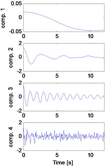
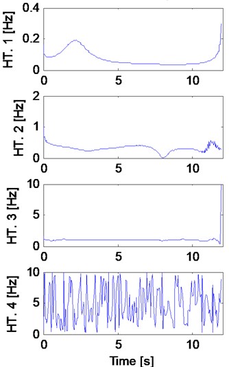
Fig. 7 shows the FT of the synthetic signal with three detected boundaries through EWT, shown by dashed vertical lines resulting in four frequency regions. The boundaries are detected at the lowest local minima between d (number of DOF) largest maxima. A wavelet filter is generated for each region and is used to create a sub-signal containing a separate mode. In this case, the first boundary in Fig. 7 is not between the first two frequencies resulting in a spurious first detected mode. Further, the region between the first and second boundaries contains the first two modes of the signal resulting in mixing of the first two modes. Fig. 8 shows the four detected components of the synthetic signal and the corresponding Hilbert spectrum using the EWT. The first component is non-oscillatory and represents none of the signal modes because of the incorrect detection of the first boundary. Component 2 represents both closely spaced modes without separating them. Components 3 and 4 represent modes 3 and 4 of the signal but the latter contains high-frequency noise. Performance of this method depends greatly on the correct detection of the boundaries and the scheme used for this purpose is not effective when the signal contains closely-spaced frequencies. EWT yields separate modes in time and time-frequency domains but no system parameter is extracted directly. The estimated values of the four frequencies, the peaks in FT of each output (Fig. 7) are presented in Table 1.
Fig. 7The FT of the synthetic signal using EWT where three boundaries are detected with dashed vertical lines resulting in four frequency regions
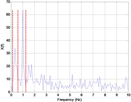
Fig. 8a) Four detected components of the synthetic signal and b) the corresponding HT using the EWT
a)
b)
4.3. Approximate Prony method
The idea of representing sequences by sums of damped exponential goes back to mathematician Gaspard de Prony as early as 1795 but was applied in the signal processing practice in the late 1980s [54-56]. Prony’s method was intended for exact representation of noncontaminated signals without any noise [57]. When applied to noisy signals the method exhibits numerical instability and inaccurate frequency and damping estimation and researchers have tried to modify and improve the performance of the method. Beylkin and Monzón [58] used the Prony’s method to efficiently approximate complex exponentials contaminated by noise. The method, called the Approximate Prony method (APM), overcomes the numerical instability of the original method and results in a more efficient approach. Potts and Tasche [59] extended the work of Beylkin and Monzón for non-damped multivariate exponential data and proposed the sparse approximate Prony method that uses a lower number of sampled data. In this research this approach is used for damped exponentials with noise.
The idea of Prony’s method is based on the fact that the solutions of homogeneous linear ordinary differential equations are sum of complex exponentials. In addition, linear differential or difference equations are transformed to a linear recurrence sequence, similar to autoregressive (AR) models. Therefore, the signal must fit in a recurrence model. The roots of the polynomial formed by the coefficients of the AR model describe the model in explicit form. In Prony’s method the signal is assumed to be sum of complex exponentials, and is decomposed into a preselected number of exponentially decaying sinusoids in the following form:
where:
αn, μn, fn, φn are the amplitude, damping exponent, frequency, and phase angle of the nth component respectively, Sn is called the residue, weight, phasor (in electronics) or complex coefficient, and zn is called the pole corresponding to the nth component of the signal since they are the roots of a polynomial to be described in the next paragraph.
Using the number of signal components, D, and the signal length N, an integer L is chosen in the range D<L<N/2 depending on the types of the signal and its noise content and a data Hankel matrix (a flip of Toeplitz matrix), F1, and a data vector, v, are formed similar to AR model of order L as follows:
Next, the following equation is solved to find the constant complex coefficients vector c=[cL,…,c1]T:
Therefore, assuming N>2L:
where F+1 is the Moore-Penrose pseudoinverse of F1 used to solve the linear least squares problem defined by Eq. (20). Coefficients of the recurrence sequence, ci, are used to form an Lth order complex polynomial as follows:
Roots of Eq. (22) are the estimates of poles defined in Eq. (17). In noiseless situations, only D non-zero coefficients are found by Eq. (21) that completely describe the signal content. However, with the existence of noise, D roots are chosen that best match the signal components among possibly more than L non-zero roots. Next, using the D selected roots, the N-L-1 by D Vandermonde data matrix or the matrix of found exponential columns is formed and used to find the complex coefficients (residues) vector S to be used in Eq. (15):
The main challenge in this method is the selection of the roots that are related to signal components and not spurious modes.
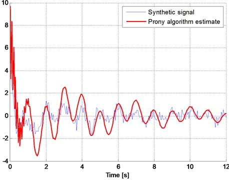
Table 1 presents the estimated values of the four frequencies and their corresponding damping exponents. This method tends to distinguish the two closely-spaced frequencies but not accurately at 0.2 and 0.55 Hz compared with the actual values of 0.3 and 0.5 Hz. The inaccuracy is reflected in the estimated signal shown in Fig. 9 which does not replicate the original signal accurately. Further, there exists a spurious frequency at 9.81 Hz that contributes to the high-frequency oscillation during the first second of the estimated signal, with a high damping exponent that contributes to the fast dissipation of this mode as seen in Fig. 9.
Fig. 9Comparison of the signal estimated by the AP method with the original synthetic signal
4.4. Matrix Pencil method
Similar to the AP method, the Matrix Pencil (MP) method is also used to decompose the signal into a preselected number of exponentially decaying sinusoids. For any given signal, an integer L called the pencil parameter is chosen in the range D<L<N/2 and two data matrices F1 and F2 of size (N-L)×L are formed similar to data matrices in the Prony’s method but with a delay of one time increment as follows [60, 61]:
Parameter L is chosen to minimize the effect of noise in the data as explained in the AP method. Assuming linear approximation, matrices F1 and F2 are written in the following form:
where:
where ZL and ZR are (N-L)×D and D×L matrices, respectively, and Si and zi are defined by Eqs. (16) and (17). The Pencil of matrices F1 and F2 is:
Eq. (32) shows that if λ is equal to any of poles (zi), it is also an eigenvalue of the pencil of matrices F1, F2. As such, finding eigenvalues is equivalent to finding the poles of the signal as:
where superscript “+” denotes the pseudoinverse of the rectangular matrix defined as:
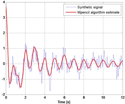
Table 1 presents the estimated values of the four frequencies and their corresponding damping exponents. This method distinguishes the two closely-spaced frequencies accurately at 0.32 Hz and 0.55 Hz compared with the actual values of 0.3 Hz and 0.5 Hz and generates no spurious solutions. Fig. 10 shows comparison of the signal estimated by the MP method with the original synthetic signal. The MP method results in a better match in time domain compared with the AP method confirming the earlier assertion by Sarkar and Pereira 1995 that MP works better in the presence of noise without actually comparing the two methods.
Fig. 10Comparison of the signal estimated by the MP method with the original synthetic signal
4.5. Esprit method
Estimation of Signal Parameters by Rotational Invariance Technique (ESPRIT) [62] explores the rotational invariance property in the signal subspace. The guiding principle of ESPRIT is closely related to that of Matrix Pencil [63, 64]. ESPRIT estimates the frequencies ωn(i=1,…,D) as arg(vi) (for argument or phase angle) where vis are the eigenvalues of the matrix Φ as follows:
in which S1 and S2 are data matrices similar to F1 and F2 defined by Eqs. (29) and (30).
The frequencies estimated by this approach for the synthetic signal are presented in Table 1. ESPRIT is also unable to detect the closely spaced frequencies.
5. Statistical performance study
In addition to studying the performance of each method on a selected synthetic signal, the Monte Carlo statistical approach is used to investigate the effect of the random noise in the signal. Table 2 presents the average errors for the estimated parameters using 100 different trials for four different signal lengths of 3, 6, 9, and 12 sec and four different signal-to-noise ratios of 1, 3, 6, and 9. For a parameter vector Pr and estimated vector ~Pr the error values in Table 2 are averages of root mean square (rms) of the error vector divided by root mean square of original parameters vector:
The results show that generally all methods yield higher errors for shorter signal length and lower SNR ratios as expected. Also, non-parametric signal processing methods perform considerably better than parametric methods for longer signal lengths. But, with the reduction in the signal length the performance of all methods deteriorate.
On average, non-parametric methods seem to provide more accurate results but are highly affected by both signal length and SNR ratio while parametric methods show more sensitivity to SNR ratio than the signal length. Moreover, using the same SNR ratio, all parametric methods yield almost the same error value. In contrast, non-parametric methods are more sensitive to the SNR ratio.
Because of the performance consistency, parametric methods appear to be more suitable for signals with a lower number of sample points. The almost constant error values for frequency estimation under different signal length and SNR values in parametric methods suggest the existence of a methodological error in these methods.
Table 2Average error for parameter estimations in 100 tests*
FT | PSD | MUSIC | ESPRIT | Matrix pencil | Prony | ||||
Freq. | Freq. | Freq. | Freq. | Freq. | Damp. | Freq. | Damp. | ||
Signal length 3 sec | SNR 1 | 3.44 | 4.07 | 5.02 | 4.07 | 5.14 | 23.22 | 5.30 | 16.59 |
SNR 3 | 3.17 | 3.50 | 4.74 | 3.50 | 4.54 | 7.67 | 4.68 | 7.47 | |
SNR 6 | 2.47 | 3.02 | 4.81 | 3.02 | 3.95 | 9.64 | 4.07 | 9.95 | |
SNR 9 | 2.17 | 3.19 | 4.19 | 3.19 | 3.90 | 6.96 | 4.02 | 7.07 | |
Signal length 6 sec | SNR 1 | 2.67 | 3.67 | 4.52 | 3.67 | 4.55 | 3.11 | 4.69 | 2.87 |
SNR 3 | 2.66 | 3.31 | 4.36 | 3.31 | 4.16 | 3.10 | 4.28 | 3.02 | |
SNR 6 | 1.52 | 2.89 | 3.96 | 2.89 | 4.06 | 4.86 | 4.18 | 4.76 | |
SNR 9 | 1.98 | 3.28 | 3.88 | 3.28 | 3.67 | 1.80 | 3.78 | 1.83 | |
Signal length 9 sec | SNR 1 | 1.64 | 3.71 | 3.73 | 3.71 | 4.37 | 3.25 | 4.50 | 3.23 |
SNR 3 | 0.79 | 2.98 | 3.55 | 2.98 | 3.80 | 2.83 | 3.91 | 2.57 | |
SNR 6 | 0.77 | 2.43 | 2.62 | 2.43 | 3.48 | 4.45 | 3.58 | 3.32 | |
SNR 9 | 0.85 | 2.42 | 2.98 | 2.42 | 3.06 | 4.81 | 3.15 | 2.81 | |
Signal length 12 sec | SNR 1 | 1.17 | 3.44 | 3.44 | 3.44 | 4.43 | 4.87 | 4.56 | 4.69 |
SNR 3 | 0.50 | 3.22 | 3.75 | 3.22 | 3.70 | 4.10 | 3.81 | 4.13 | |
SNR 6 | 0.36 | 2.35 | 3.30 | 2.35 | 3.83 | 3.89 | 3.94 | 3.74 | |
SNR 9 | 0.51 | 2.81 | 3.06 | 2.81 | 3.77 | 3.60 | 3.89 | 3.65 | |
*Only the methods providing parameter values are considered in the table | |||||||||
6. Conclusions
While detection of the stationary content of the signals have been vastly studied over many decades non-stationary and specifically exponentially damped content detection is a relatively newer concept. However, in virtually all real systems the responses are damped and non-stationary. Accurate detection of the structural properties such as frequency and damping coefficient is of a great value in SHM. In this paper different signal processing methods were reviewed and their performances compared. The performance of nonparametric methods is highly affected by the length of sample signal and, while that of parametric methods is highly affected by SNR. This research has provided the impetus to develop a new and more powerful signal processing technique for non-stationary signals contaminated with noise and closely-spaced frequencies.
References
-
Nigro M. B., Pakzad S. N., Dorvash S. Localized structural damage detection: a change point analysis. Computer-Aided Civil and Infrastructure Engineering, Vol. 29, Issue 6, 2014, p. 416-432.
-
Su W. C., Huang C. S., Chen Ch, Liu C. Y., Huang H. C., Le Q. T. Identifying the modal parameters of a structure from ambient vibration data via the stationary wavelet packet. Computer-Aided Civil and Infrastructure Engineering, Vol. 29, Issue 10, 2014, p. 738-57.
-
Story B. A., Fry G. T. A structural impairment detection system using competitive arrays of artificial neural networks. Computer-Aided Civil and Infrastructure Engineering, Vol. 29, Issue 3, 2014, p. 180-90.
-
Butcher J. B., Day C. R., Austin J. C., Haycock P. W., Verstraeten D., Schrauwen B. Defect detection in reinforced concrete using random neural architectures. Computer-Aided Civil and Infrastructure Engineering, Vol. 29, Issue 3, 2013, p. 191-207.
-
O’Byrne M., Schoefs F., Pakrashi V., Ghosh B. Regionally enhanced multi-phase segmentation technique for damaged surfaces. Computer-Aided Civil and Infrastructure Engineering, Vol. 29, Issue 9, 2014, p. 644-658.
-
Yeum C. M., Dyke S. J. Vision based automated crack detection for bridge inspection. Computer-Aided Civil and Infrastructure Engineering, Vol. 30, Issue 10, 2015, p. 759-770.
-
Tondini N., Bursi O. S., Bonelli A., Fassin M. Capabilities of a fiber bragg grating sensor system to monitor the inelastic response of concrete sections in new tunnel linings subjected to earthquake loading. Computer-Aided Civil and Infrastructure Engineering, Vol. 30, Issue 8, 2015, p. 636-653.
-
Foti D., Gattulli V., Potenza F. Output-only identification and finite element updating by dynamic testing in unfavorable operative conditions of a seismically damaged building. Computer-Aided Civil and Infrastructure Engineering, Vol. 29, Issue 9, 2014, p. 659-675.
-
Khalid M., Yusof R., Joshani M., Joshani M., Selamat H. Nonlinear identification of a magneto-rheological damper based on dynamic neural networks. Computer-Aided Civil and Infrastructure Engineering, Vol. 29, Issue 3, 2014, p. 221-233.
-
Bursi O. S., Ceravolo R., Kumar A., Abbiati G. Identification, model updating and validation of a steel twin deck curved cable-stayed footbridge. Computer-Aided Civil and Infrastructure Engineering, Vol. 29, Issue 9, 2014, p. 703-722.
-
Torbol M. Real-time frequency-domain decomposition for structural health monitoring using general-purpose graphic processing unit. MICE Computer-Aided Civil and Infrastructure Engineering, Vol. 29, Issue 9, 2014, p. 689-702.
-
Huang Y., Beck J. L., Wu S., Li H. Robust Bayesian compressive sensing for signals in structural health monitoring. Computer-Aided Civil and Infrastructure Engineering, Vol. 29, Issue 3, 2014, p. 160-179.
-
Ghosh-Dastidar S., Adeli H. Wavelet-clustering-neural network model for freeway incident detection. Computer-Aided Civil and Infrastructure Engineering, Vol. 18, Issue 5, 2003, p. 325-338.
-
Dharia A., Adeli H. Neural network model for rapid forecasting of freeway link travel time. Engineering Applications of Artificial Intelligence, Vol. 16, Issues 7-8, 2003, p. 607-613.
-
Jiang X., Adeli H. Object-oriented model for freeway work zone capacity and queue delay estimation. Computer-Aided Civil and Infrastructure Engineering, Vol. 19, Issue 2, 2004, p. 144-156.
-
Jiang X., Adeli H. Wavelet packet-autocorrelation function method for traffic flow pattern analysis. Computer-Aided Civil and Infrastructure Engineering, Vol. 19, Issue 6, 2004, p. 324-337.
-
Jiang X., Adeli H. Clustering-neural network models for freeway work zone capacity estimation. International Journal of Neural Systems, Vol. 14, Issue 3, 2004, p. 147-163.
-
Adeli H., Ghosh-Dastidar S. Mesoscopic-wavelet freeway work zone flow and congestion feature extraction model. Journal of Transportation Engineering, ASCE, Vol. 130, Issue 1, 2004, p. 94-103.
-
Castillo E., Calvino A., Nogal M., Lo H. K. On the probabilistic and physical consistency of traffic random variables and models. Computer-Aided Civil and Infrastructure Engineering, Vol. 29, Issue 7, 2014, p. 496-517.
-
Ngoduy D., Wilson R. E. Multi-anticipative non-local macroscopic traffic model. Computer-Aided Civil and Infrastructure Engineering, Vol. 29, Issue 4, 2014, p. 248-263.
-
Haijema R., Hendrix E. M. T. Traffic responsive control of intersections with predicted arrival times: a Markovian approach. Computer-Aided Civil and Infrastructure Engineering, Vol. 29, Issue 2, 2014, p. 123-139.
-
Sankari Z., Adeli H. HeartSaver: A mobile cardiac monitoring system for auto-detection of atrial fibrillation, myocardial infarction and atrio-ventricular block. Computers in Biology and Medicine, Vol. 41, Issue 4, 2011, p. 211-220.
-
Martis R. J., Acharya U. R., Adeli H. Current methods in electrocardiogram characterization. Computers in Biology and Medicine, Vol. 48, 2014, p. 133-149.
-
Martis R. J., Rajendra Acharya U., Adeli H., Tan J. H., Tong L., Chua C. K., Loon T. C., Jie S. Y. W. Computer aided diagnosis of atrial arrhythmia using dimensionality reduction methods on transform domain representation. Biomedical Signal Processing and Control, Vol. 13, 2014, p. 295-305.
-
Zhang C., Wang H., Wang H., Wu M. EEG-based expert system using complexity measures and probability density function control in alpha sub-band. Integrated Computer-Aided Engineering, Vol. 20, Issue 4, 2013, p. 391-405.
-
Yuan Q., Zhou W., Yuan S., Li X., Wang J., Jia G. Epileptic EEG Classification based on kernel sparse representation. International Journal of Neural Systems, Vol. 24, Issue 4, 2014, p. 1450015.
-
Yuan S., Zhou W., Yuan Q., Li X., Wu Q., Zhao X., Wang J. Kernel collaborative representation-based automatic seizure detection in intracranial EEG. International Journal of Neural Systems, Vol. 25, Issue 2, 2015, p. 1550003-1550016.
-
Lin L. C., Ouyang C. S., Chiang C. T., Yang R. C., Wu R. C., Wu H. C. Early prediction of medication refractoriness in children with idiopathic epilepsy based on scalp EEG analysis. International Journal of Neural Systems, Vol. 24, Issue 7, 2014, p. 1450023-1450039.
-
Kwon M., Kavuri Sri S., Lee M. Action-perception cycle learning for incremental emotion recognition in a movie clip using 3D fuzzy GIST based on visual and EEG signals. Integrated Computer-Aided Engineering, Vol. 21, Issue 3, 2014, p. 295-310.
-
Wang H., Zhang C., Shi T., Wang F., Ma S. Real-time EEG-based detection of fatigue driving danger for accident prediction. International Journal of Neural Systems, Vol. 25, Issue 2, 2015, p. 1550002-1550016.
-
Cabessa J., Siegelmann H. T. The super-turing computational power of evolving recurrent neural networks. International Journal of Neural Systems, Vol. 24, Issue 8, 2014, p. 1450029-1450051.
-
Adeli H., Gere J., Weaver W. Jr. Algorithms for nonlinear structural dynamics. Journal of Structural Division, ASCE, Vol. 104, Issue ST2, 1978, p. 263-280.
-
Ghodrati Amiri G., Abdolahi Rad A., Khanmohamadi Hazaveh N. Wavelet based method for generating non-stationary artificial pulse-like near-fault ground motions. Computer-Aided Civil and Infrastructure Engineering, Vol. 29, Issue 10, 2014, p. 758-770.
-
Dai H., Wang W. An adaptive wavelet frame neural network method for efficient reliability analysis. Computer-Aided Civil and Infrastructure Engineering, Vol. 29, Issue 10, 2014, p. 801-814.
-
Amini F., Zabihi-Samani M. A Wavelet-based adaptive pole assignment method for structural control. Computer-Aided Civil and Infrastructure Engineering, Vol. 29, Issue 6, 2014, p. 464-477.
-
Su W. C., Liu C. Y., Huang C. S. Identification of instantaneous modal parameter of time-varying systems via a wavelet-based approach and its application. Computer-aided Civil and Infrastructure Engineering, Vol. 29, Issue 4, 2014, p. 279-298.
-
Kodogiannis V. S., Amina M., Petrounias I. A clustering-based fuzzy-wavelet neural network model for short-term load forecasting. International Journal of Neural Systems, Vol. 23, Issue 5, 2013, p. 1350024-1350043.
-
Hsu W. Y. Assembling a multi-feature EEG classifier for left-right motor data using wavelet-based fuzzy approximate entropy for improved accuracy. International Journal of Neural Systems, Vol. 25, Issue 8, 2015, p. 1550037-1550050.
-
Vahabi Z., Amirfattahi R., Ghassemi F., Shayegh F. Online epileptic seizure prediction using wavelet-based bi-phase correlation of electrical signal tomography. International Journal of Neural Systems, Vol. 25, Issue 6, 2015, p. 1550028-1550050.
-
Jiang X., Adeli H. Dynamic wavelet neural network model for traffic flow forecasting. Journal of Transportation Engineering, ASCE, Vol. 131, Issue 10, 2005, p. 771-779.
-
Adeli H., Karim A. Wavelets in Intelligent Transportation Systems. John Wiley and Sons, West Sussex, United Kingdom, 2005.
-
Ghosh-Dastidar S., Adeli H. Neural network-wavelet micro-simulation model for delay and queue length estimation at freeway work zones. Journal of Transportation Engineering, ASCE, Vol. 132, Issue 4, 2006, p. 331-341.
-
Adeli H., Jiang X. Intelligent Infrastructure – Neural Networks, Wavelets, and Chaos Theory for Intelligent Transportation Systems and Smart Structures. CRC Press, Taylor and Francis, Boca Raton, Florida, 2009.
-
Katicha S. W., Flintsch G., Ferne B., Bryce J. Wavelet denoising of tsd deflection slope measurements for improved pavement structural evaluation. Computer-Aided Civil and Infrastructure Engineering, Vol. 29, Issue 6, 2014, p. 399-415.
-
Jiang X., Mahadevan S., Adeli H. Bayesian wavelet packet denoising for structural system identification. Structural Control and Health Monitoring, Vol. 14, Issue 2, 2007, p. 333-356.
-
Perez G., Conci A., Moreno A. B., Hernandez-Tamames J. A. Rician noise attenuation in the wavelet packet transformed domain for brain MRI. Integrated Computer-Aided Engineering, Vol. 21, Issue 2, 2014, p. 163-175.
-
Huang N. E., Shen Z., Long S. R., Wu M. C., Shih H. H., Zheng Q., Yen N., Tung C. C., Liu H. H. The empirical mode decomposition and the Hilbert spectrum for nonlinear and non-stationary time series analysis. Proceedings of the Royal Society of London A: Mathematical, Physical and Engineering Sciences, Vol. 454, Issue 1971, 1998, p. 903-995.
-
Gabor D. Theory of communication. Proceedings of the IEEE, Vol. 93, Issue 3, 1946, p. 429-457.
-
Pisarenko V. F. The retrieval of harmonics from a covariance function. Geophysical Journal of the Royal Astronomical Society, Vol. 33, Issue 3, 1973, p. 347-366.
-
Schmidt R. O. Multiple emitter location and signal parameter estimation. IEEE Transactions on Antennas and Propagation, Vol. 34, Issue 3, 1986, p. 276-280.
-
Nadakuditi R. R., Edelman A. Sample eigenvalue based detection of high-dimensional signals in white noise using relatively few samples (Technical Report). IEEE Transactions on Signal Processing, Vol. 56, Issue 7, 2008.
-
Bienvenu G. Influence of the spatial coherence of the background noise on high resolution passive methods. Acoustics, Speech, and Signal Processing, IEEE International Conference on ICASSP, 1979, p. 306-309.
-
Giles J. Empirical wavelet transform. IEEE Transactions on Signal Processing, Vol. 61, Issue 16, 2013, p. 3999-4010.
-
Marple S. L. Digital Spectral Analysis with Applications. McGraw-Hill, New York, 1987.
-
Hauer J. F., Demeure C. J., Scharf L. L. Initial results in Prony analysis of power system response signals. IEEE Transactions on Power Systems, Vol. 5, Issue 1, 1990, p. 80-89.
-
Kundu D., Mitra A. Different Non iterative methods to estimate sinusoidal frequencies: a numerical comparison. Journal of Statistical Computation and Simulations, Vol. 62, Issue 1, 1998, p. 9-28.
-
Potts D., Tasche M. Parameter estimation for exponential sums by approximate Prony method. Signal Processing, Vol. 90, Issue 5, 2010, p. 1631-1642.
-
Beylkin G., Monzón L. On approximation of functions by exponential sums. Applied and Computational Harmonic Analysis, Vol. 19, Issue 1, 2005, p. 17-48.
-
Potts D., Tasche M. Parameter estimation for nonincreasing exponential sums by Prony-like methods. Linear Algebra and its Applications, Vol. 439, Issue 4, 2013.
-
Hua Y., Sarkar T. K. Matrix pencil method for estimating parameters of exponentially damped/undamped sinusoids in noise. Acoustics, IEEE Transactions on Speech and Signal Processing, Vol. 38, Issue 5, 1990, p. 814-824.
-
Sarkar T. K., Pereira O. Using the matrix pencil method to estimate the parameters of a sum of complex exponentials. IEEE Antennas and Propagation Magazine, Vol. 37, Issue 1, 1995, p. 48-55.
-
Paulraj A., Roy R., Kailath T. Estimation of signal parameters via rotational invariance techniques – ESPRIT. 19th Asilomar Conference on Circuits, Systems and Computers, Vol. 6, Issue 8, 1985, p. 83-89.
-
Khan Z. I., Awang R. A., Sulaiman A. A., Jusoh M. H., Baba N. H., Kamal M. M. D., Khan N. I. Performance analysis for estimation of signal parameters via rotational invariance technique (ESPRIT) in estimating direction of arrival for linear array antenna. RF and Microwave Conference, IEEE International, Vol. 2, Issue 4, 2008, p. 530-533.
-
Hung C. J., Chen C. H. New algorithm for fast direction-of-arrival estimation using the shrinking signal subspace and the noise pseudo-eigenvector. Radar, Sonar and Navigation, Vol. 4, Issue 4, 2010, p. 604-610.

