Structural dynamic model updating based on Kriging model using frequency response data

1. Introduction

Structural dynamic Model Updating Method has been widely used in civil engineering, aerospace engineering and other fields during the past four decades. In recent years, mainly two model updating methods of structural dynamics are studied: the modal parameters based method [1] and the frequency response function (FRF) based method [2]. The modal parameter based method has been widely applied in many practical applications, however, fewer studies focus on the FRF based method. The FRF based method has at least four advantages over the modal parameter based method:1) It can take advantage of the measured vibration data directly without data transformation, which may introduce algorithm or numerical errors; 2) It avoids modal analysis, and is suitable for the structure with dense mode; 3) FRF can provide more data that each response curve can be used as an objective function for model updating [3]; 4) In some cases, the error of modal identification might be greater than the error of structure modeling [4], which is the main error of model updating. The FRF based model updating is worth to be thoroughly studied, thereby FRF based method is gaining more and more attention.

Hemez and Brown [5] introduced the FRF based model updating method, its advantages and limitations in engineering application were also described. García-Palencia et al. [6] and Fei et al. [7] performed their proposed model updating method on the UCF Benchmark structure and GARTEUR truss structure by using FRF data respectively, and the FRF curves of experimental and updated model tended to coincidence. In addition, many studies on damage/parameter identification and health monitoring of structures are based on the FRF model updating [8-11].

The model updating process is usually formulated as minimizing the differences between the experimental model and the finite element model (analytical model), so it is essentially an optimization problem. But the traditional sensitivity-based optimization methods have at least two disadvantages: first, the requirement of sensitivity analysis may be computation expensive or even, the sensitivity results may not be readily obtained and; second, when numerous iterations are required for convergence of the optimization algorithm, especially to modern intelligent algorithms that huge computational cost may be needed. Since the time-consuming finite element analysis codes will be run at least once per iteration, this will be a challenge for structural dynamic model updating.

The recently developed metamodel techniques bridge the gap between the intelligent algorithm and practical applications. They use an approximate model to approximate the relationship between the input and output of a black-box system, other information of the system is not required, so the existing commercial and in-house finite element analysis codes can be integrated directly, and additionally it is suitable for parallel computing. Once the metamodel is constructed and validated, it can be used to replace the exact finite element analysis (FEA) to perform model updating. Due to the low computational cost of metamodel, the modern intelligent optimization method can be applied to increase the probability of getting the global optimum. Therefore, the potential of metamodel techniques is indisputable.

Three kinds of metamodel are widely been used: response surface methodology (RSM), Kriging method and radial basis function (RBF), and they have been well studied in some fields, such as structural static model updating [12], structural dynamic model updating based on modal parameters [13], structural damage identification [14,15], structural reliability analysis [16]. Some researcher also gave the comparison [17, 18] and recommendation [19] of the main metamodels. However, it is hard to find any studies which focused on their applications in structural dynamic model updating based on FRF. As one of the main metamodels, Kriging model is usually more accurate than traditional RSM. Khodaparast et al. [20] investigated the interval model updating based on Kriging method, and presented its good accuracy through an example of a beam positions. Govers et al. [21] carried out stochastic model updating of the DLR AIRMOD structure by two methods based on Kriging model. Liu et al. [22] updated the structural model of an arch bridge by using a two-level method based on Kriging model. Therefore, the Kriging method should receive attention in dynamic model updating.

In this article, the FRF based model updating is studied based on Kriging model, which is constructed based on the DOE results of input-output of structural dynamics, whose output response is based on acceleration FRF (AFRF) data. Two examples of composite structure are discussed, the model updating results with less error are obtained based on Kriging model, the effectiveness of the proposed approach is demonstrated.

2. AFRF based model updating

As one kind of FRF, the basic theory of AFRF comes from n degree of freedom (DOF) dynamic system, whose motion equation is given as:

where $\mathbf{M}$, $\mathbf{C}$ and $\mathbf{K}$ are $n\times n$ mass matrix, damping matrix and stiffness matrix of the system, respectively, $\mathbf{F}\left(={\mathbf{F}}_0{e}^{i\omega t}\right)$ is excitation vector, $\mathbf{x}$ is displacement vector.

When applying simple harmonic excitation, the AFRF of the system can be obtained as:

where $\omega$ is the excitation frequency.

When creating finite element model (FEM), some parameters usually have deviations from those of the experimental model, and the deviations are considered as modeling errors, which result in errors of mass, damping or stiffness of the FEM, as a consequence, AFRF differences between FEM and experimental model arise from the deviations.

Model updating aims primarily to reduce the FEM error from the experimental model by modifying some parameters of the FEM. In AFRF based model updating, AFRF curves (both FEM and experimental model) at certain DOFs are observed and given as inconsistent curves, which are taken as updating objectives. In order to make the FEM AFRF coincide with experimental AFRF by model updating, an optimization problem is formulated and its solution is taken as the updated values of the parameters. The objective function of the optimization problem is established by using the differences between the analytical and experimental AFRF based data.

In this study, the errors between the coupled AFRF curves at each frequency point are involved in creating the objective function as follows:

where $np$ is the number of selected observation DOFs, $nf$ is the number of the selected frequency points of AFRF, $A_t^n\left({\omega }_i\right)$ is acceleration amplitude at the selected frequency point of the experimental model, $A_a^n\left({\omega }_i\right)$ is the corresponding acceleration amplitude of the FEM, ${\omega }_i$is the selected frequency points.

The optimization problem can be formulated in the following form:

where $x_i$ is the design variables of the FEM, $x_{iL}$ and $x_{iU}$ is the lower and upper bound of the design variables.

3. Constructing Kriging model

This section will introduce the construction method of Kriging model. The Kriging model includes a linear regression part and a nonparametric part that can be described as:

where $\mathbf{\beta }$ is the coefficient vector of the regression, $\mathbf{f}\left(x\right)$ is the polynomial vector of variable $\mathbf{x}$, $z\left(\mathbf{x}\right)$ is the realization of the stochastic process whose mean is zero.

The $f\left(x\right)$ provides a ‘global’ approximation of the Kriging model, $z\left(x\right)$ is an approximation of local deviation of the Kriging model, and $z\left(x\right)$ follows normal distribution $N\left(0,{\sigma }_z^{}\right)$ with nonzero covariance, whose expression is given as follows:

where ${\sigma }_z$ is the variance of $z\left(x\right)$, $x_i$ and $x_j$ are any two of the training samples, $\mathbf{R}$ is a symmetry matrix composed by $R_{ij}\left(x_i,x_j\right)$. In this study, the training samples come from DOE results.

$R_{ij}$ is the correlation function, which can characterize the correlation between training points, and it can affect the approximation accuracy of the Kriging model. The form of $R_{ij}$ as follows:

where $N_v$ is the number of design variables, ${\theta }_k$ is the coefficient of correlation, $x_i^k$ and $x_j^k$ are the $k$th component of $x_i$ and $x_j$ respectively.

In this study, the Gaussian correlation function is taken as the kernel function, which has a widely application with the following form:

where, the detailed derivation process of ${\theta }_k$ and ${\sigma }_z$ can be found in reference [23]. The values of ${\theta }_k$ and ${\sigma }_z$ can be obtained by solving the maximum likelihood estimated problem as follows:

where $\left|\mathbf{R}\right|$ is the determinant of $\mathbf{R}$, $N_s$ is the number of training samples, ${\sigma }_z$ is the function of ${\theta }_k$ and $\mathbf{R}$.

In most cases, a constant term in Eq. (5) is enough to describe the trends of the output response, which corresponding to the value of objective function in this study. Accordingly, any output response $y\left(x\right)$ can be dealt with stochastic process with normal distribution when constructing Kriging model. A constant term is used to instead the polynomial term in following discussion.

When the Kriging model is obtained, the unbiased estimation of $\widehat{y}\left(x_0\right)$ of $x_0$ can be expressed as:

where $\mathbf{Y}$ is a column vector composed by output response of training samples, $\mathbf{f}$ is a column vector by $f\left(x\right)$ of training samples, $r\left(x_0\right)$ is relevant vector composed by training samples and predict point $x_0$:

In short, the Kriging model will be determined when the values of ${\theta }_k$ are known.

4. Model updating procedure

According to the previous two sections, Kriging model is introduced to the AFRF based model updating process, where the FEA is replaced by the Kriging model during the optimization process. The optimization results of input variables of Kriging model are taken as the updated values of input variables of model updating, and the FEM can be modified by using the results. Accordingly, after model updating, the frequency response curves of FEM tend to coincide with the experimental curves in the selected observation DOFs.

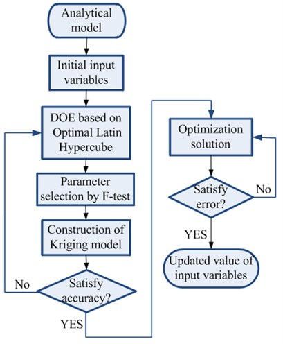
Generally, analytical model has many parameters, and some of them should be selected as initial input variables, which are taken as the DOE factors. And the design matrix of DOE is generated by Optimal Latin Hypercube sampling method in this study. Then the Kriging model is created based on the DOE results, whose sampling points are taken as training points for solving basic parameters ${\theta }_k$ of Kriging model.

In most cases, nevertheless, different input variables (FEM parameters) have different sensitivity to the output response (AFRF based data). When solving the optimization problem for model updating, the optimization algorithm cannot optimize the insensitive parameters effectively. In this study, the input variables of Kriging model only include the sensitive ones. Specifically, the F-test method [24] is used to estimate the sensitivity of the factors based on DOE results. If the factors have significant influence on the DOE response (based on Eq. (3)), they will be chosen as the input variables of Kriging model. Correspondingly, the training samples only include the selected variables and response of DOE results. Furthermore, the accuracy of the constructed Kriging model will be checked.

Finally, the optimized values of input variables are obtained after optimization based on the Kriging model. The FEM is updated by the optimized input variables until the error of analytical AFRF curve is satisfied. The flow chart of the proposed procedure of model updating can be given as Fig. 1.

Fig. 1Flow chart of the procedure of model updating

5. Numerical study

In this section, two numerical examples are performed to demonstrate the effectiveness of the proposed method. The two examples are representative in practical engineering: plate structure and solar array structure.

5.1. Example 1: honeycomb sandwich plate

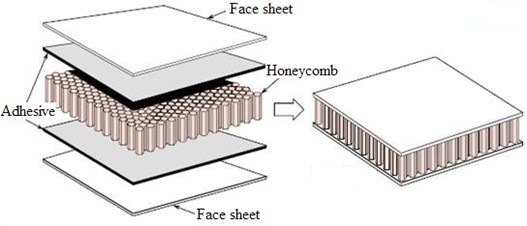
Honeycomb sandwich structure has many advantages of mechanical properties, so it is widely applied in the aerospace industry and some other lightweight needed industry. Honeycomb sandwich plate shown as Fig. 2 typically consists of 5 parts: two thin face sheets, one much thicker lightweight honeycomb-core, and two adhesive layers combine the core and faces.

Fig. 2The honeycomb sandwich structure

In this section, the model updating of a honeycomb sandwich plate with composite skins and aluminum core is studied. The FEM is constructed by 150 shell elements shown as Fig. 3 without showing the thickness, its dimension is 516×351×10 mm with 11 layers totally. As shown in Fig. 3, point a and c are the positions of fixed constraint, point b is the observation DOF, and point d is the excitation DOF. Also, Fig. 3 shows the dimension of the honeycomb cell of the aluminum core that used in this study. The details of thickness and angles of each layer are given in Table 1.

Fig. 3The FEM of honeycomb sandwich plate

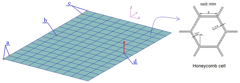
Table 1Thickness and angles of each layer

Layer	Material	Thickness (mm)	Angle
1	Carbon fiber	0.1	–45°
2	Carbon fiber	0.1	90°
3	Carbon fiber	0.1	45°
4	Carbon fiber	0.1	90°
5	Adhesive	0.15	0°
6	Honeycomb core	8.9	0°
7	Adhesive	0.15	0°
8	Carbon fiber	0.1	90°
9	Carbon fiber	0.1	45°
10	Carbon fiber	0.1	90°
11	Carbon fiber	0.1	–45°

The excitation is a 1 N harmonic force (in $Z$ direction) at point d under 3 % critical damping, and the measurement of acceleration frequency response in $Z$ direction of the point $b$. The optimization objective (based on Eq. (3)) for model updating is created based on the response error of acceleration amplitude between the experimental model and the analytical model.

5.1.1. Experimental model and analytical model

The honeycomb sandwich plate usually has a honeycomb core with large numbers of honeycomb cells as shown in Fig. 3. It is difficult to simulate and analyze the real honeycomb core with numerous cells. Therefore, in order to simplify the honeycomb core based on the honeycomb cells, three kinds of equivalent theories [25, 26] are commonly been used: sandwich plate theory, honeycomb plate theory and equivalent plate theory.

The first theory is a classic commonly method, which is adopted in this study, then the properties of the honeycomb core are considered as 2-dimension orthotropic material after equivalent. The carbon fiber is also 2-dimension orthotropic material. The properties of the two materials are summarized in Table 2 in details. In addition, the adhesive layer is considered as isotropic material, whose Young’s modulus $E=$7×10⁹ N/m², Poisson ratio $\mu =$0.3, and density $\rho =$1500 kg/m³.

As can be seen in Table 1 and 2, there are many parameters of the honeycomb sandwich plate, obviously, it is difficult to update every parameter, so it is better to select the parameters (prone to error) before model updating. Actually, the honeycomb core is an equivalent structure when establishing the FEM, and the thickness of the adhesive is difficult to control and measured. Hence, the initial input variables of the FEM for model updating and DOE come from the parameters of the honeycomb core and adhesive, the selected parameters are listed in Table 3.

For this example, the analytical model and experimental model are created based on the FEM described above. The model with exact parameter values (equivalent values or nominal values) is taken as ‘experimental’ model. The ‘analytical’ model is constructed by introduced parameter error to the ‘experimental’ model, and then the analytical model exist error from the experimental model. The parameter values of the ‘analytical’ model are considered as the initial values. Table 3 lists the parameters which will be taken as input variables of DOE.

Table 2Properties of the carbon fiber and equivalent honeycomb core

Material properties		Carbon fiber	Equivalent core
Elastic modulus	$E_x$ (Pa)	1.3×1011	0.16×106
	$E_y$ (Pa)	1×1010	0.16×106
Shear modulus	$G_{xy}$ (Pa)	5.2×109	0.06×106
	$G_{xz}$ (Pa)	4.9×109	0.16×106
	$G_{yz}$ (Pa)	3.5×109	0.23×106
Density (kg/m3)		1560	31

Table 3Parameter values of analytical model of example 1

Material name	Properties name	Initial value	Exact value	Error
Honeycomb core	$E_x$ (MPa)	0.128	0.16	–20 %
	$E_y$(MPa)	0.192	0.16	+20 %
	$G_{xy}$ (MPa)	0.048	0.06	–20 %
	$G_{xz}$ (MPa)	0.192	0.16	+20 %
	$G_{yz}$ (MPa)	0.276	0.23	+20 %
Adhesive	$E$ (MPa)	5600	7000	–20 %
	$\mu$	0.36	0.3	+20 %
	$T_1$ (mm)	0.12	0.15	–20 %
	$T_2$ (mm)	0.18	0.15	+20 %

5.1.2. DOE and parameter selection of example 1

Before performing DOE, the frequency ranges for calculated frequency points should be selected based on the AFRF curve of the experimental model. Because the error nearby the resonance peak is exacerbated when measuring, the selected ranges generally exclude the frequencies close to resonances. For this example, the frequency ranges for DOE response with 1 Hz step are selected as: 5-10 Hz, 20-40 Hz, 55 Hz, 70-80 Hz, 90-110 Hz, and 120-150 Hz. And then 91 frequency points are obtained. Additionally, in order to take into account, the noise contaminated experimental data, 10 % random noise is added to the AFRF of the experimental model.

The DOE is performed in the level of ±40 % initial values of every parameter in Table 3, the parameters of which are taken as factors of DOE. The value of objective function (calculated by Eq. (3) is taken as the DOE response, and then 150 sampling points are generated based on the design matrix created by Optimal Latin Hypercube method.

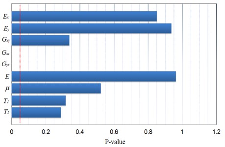
Parameters selection is performed by F-test method, which is used to check the significance of factors by P-value based on the DOE results, and significance level $P_0=$0.05 is taken as threshold, when the P-value of any factor is lower than $P_0$, it means the factor has a significant effect on the output response. This method can be formulated as:

12

$P\left\{F_A\ge F_{1-p}(f_A,f_E)\right\}=p,F_A=\frac{S_A/f_A}{S_E/f_E}~F\left(f_A,f_E\right),$

where $S_A$ is a square of error caused by factors, $S_E$ is a square of error caused by the experiment, $f_A$ and $f_E$ are the degrees of freedom of $S_A$ and $S_E$ respectively.

The P-values of the 9 factors are presented in Fig. 4. Obviously, the two factors $G_{xz}$ and $G_{yz}$ have a lower P-value than the threshold, so they are taken as input variables of model updating.

Fig. 4P-value of all factors of example 1

5.1.3. Construction and accuracy assessment of Kriging model of example 1

The Kriging model will be constructed based on the 2 selected input variables and the output response in the previous section. In other words, the generated 150 sampling points are taken as training samples for the Kriging model, whose input variables only include the 2 selected parameters. Then the unknown parameters of the Kriging model can be achieved based on the training samples. Genetic algorithm is adopted to solve the corresponding Eq. (9) and obtain the basic parameter values of ${\theta }_{xz}$ and ${\theta }_{yz}$: ${\theta }_{xz}=$25.7754, ${\theta }_{yz}=$12.8694, which are corresponding to the input variables $G_{xz}$ and $G_{yz}$ respectively.

In order to verify the accuracy of the constructed Kriging model, another 10 sampling points (different from training samples) are generated as checking points. The output response error between Kriging model and analytical model at checking points is measured by the criterion of root mean square error (RMSE), which is defined as follows:

13

$RMSE=\frac{1}{k\stackrel{-}{y}}\sqrt{\sum _{i=1}^k(y_i-{\widehat{y}}_i{)}^2},$

where $k$ is the number of checking points, $y_i$ is the response of checking points of analytical model, $\stackrel{-}{y}$ is the mean value of $y_i$, ${\widehat{y}}_i$ is the response of checking points of Kriging model.

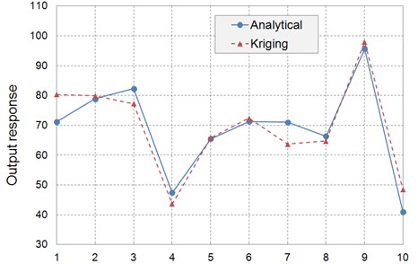
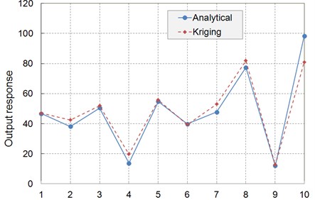
When the RMSE value is smaller than 0.1 (≥0), the accuracy is acceptable, and the smaller the value, the higher the accuracy. The response values at each checking points of Kriging model and analytical model are shown in Fig. 5. The RMSE is evaluated as about 2.2 % based on the 10 points, which means the constructed Kriging model has a good accuracy and can replace FEA during the optimization process of model updating.

5.1.4. Model updating results of example 1

Firstly, for demonstrating the importance of the F-test based parameter selection, all the 9 parameters (input variables) are involved in constructing Kriging model for comparison, Table 4 presents the optimized results after 1000 iterations solved by the Multi-island Genetic algorithm (MIGA), whose variables scope adopts ±40 % initial values of the analytical model. Obviously, the errors of parameter $E_x$ and $T_2$ are become much larger than their initial errors of analytical model, and the rest parameters are not updated effectively except $G_{xz}$. Whereas the two significant parameter $G_{xz}$ and $G_{yz}$ can be updated effectively based on the Kriging model constructed by the two, whose updated values are closer to exact values as can be seen in Table 4. So it can be considered that only the significant parameters should be selected as input variables of Kriging model for model updating.

Fig. 5The response values of checking points of example 1

Secondly, in order to demonstrate the advantage of Kriging model, a RSM model of cubic polynomial is constructed based on the same sampling points. The updated results by RSM are summarized in Table 4, parameter $G_{yz}$ is not updated effectively. So the Kriging model is more effective than the RSM model.

Table 4Update results of the 2 selected parameters

Parameters	$E_x$ (MPa)	$E_y$ (MPa)	$G_{xy}$ (MPa)	$G_{xz}$ (MPa)	$G_{yz}$ (MPa)	$E$ (MPa)	$\mu$	$T_1$ (mm)	$T_2$ (mm)
Initial value	0.128	0.192	0.048	0.192	0.276	5600	0.36	0.12	0.18
Exact value	0.16	0.16	0.06	0.16	0.23	7000	0.3	0.15	0.15
Updated	0.1194	0.1788	0.0492	0.1575	0.2639	6387.1	0.343	0.124	0.1188
Error	25.4 %	11.8 %	18.0 %	1.56 %	14.7 %	8.8 %	14.3 %	17.3 %	20.8 %
Updated by Kriging				0.1587	0.2396
Updated by RSM				0.1563	0.2923

Fig. 6Comparison between initial AFRF curve and updated AFRF curve of example 1

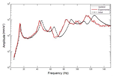
Finally, the model updating results of this example can be achieved based on the updated results of Kriging model. The initial analytical model is modified by using the two updated parameters and the rest 7 parameters keeping their initial values shown as Table 3. For comparison, three AFRF curves (in $Z$ directional) at DOF b are plotted in Fig. 6, they are updated curve, noise contaminated experimental curve and initial analytical curve respectively. As can be seen, the updated curve and the experimental curve agree well, which demonstrates the effectiveness of the proposed approach.

5.2. Example 2: solar array structure

Based on Example 1, another example much closer to engineering structure can be established as shown in Fig. 7. It is the main structure of solar array composed by hollow beams, basic honeycomb plates and joints. The dimension of beams and plates are: $D=$50 mm, $D_1=$150 mm, $D_2=$351 mm, $G=$30 mm, $D_3=$351 mm, $D_4=$516 mm, $b_1$ and $b_2$ are main beam and auxiliary beam respectively and they have the same cross section with 10 mm outer diameter. Both of the two beams are composite structure whose properties are listed in Table 5, and the honeycomb plates have the same properties of example 1 as listed in Table 1 and 2. Position $f$ is fixed constraint, e is excitation position, $P_1$ is measurement position and $P_2$ is inspection position after model updating.

Fig. 7Solar array structure and equivalent joint

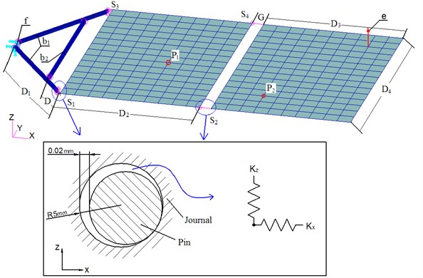
The main beam and auxiliary beam are fixed together by embedded parts. The main beam and plate are combined by joints, which also combine the two plates. Each of the joints can be considered as a spring system ($S_1-S_4$in Fig. 7) with 6 direction stiffness. The stiffness can be treated ideally as sufficiently large when the solar array is open. In most of the case, however, the $Z$-direction stiffness and $X$-direction stiffness cannot be considered as sufficiently large because of the clearance between the journal and pin as shown in Fig. 7. The two direction stiffness can be evaluated based on continuous contact force model [27] with steel material, and the values are obtained: $K_x=K_z=$5.4×10⁶ N/mm.

Table 5Thickness and angles of each layer of beams

Layer	Material	Thickness (mm)	Angle
1	Carbon fiber	0.1	–45°
2	Carbon fiber	0.1	90°
3	Carbon fiber	0.1	45°
4	Carbon fiber	0.1	90°
5	Carbon fiber	0.1	–45°

Meanwhile, the ‘experimental’ and ‘analytical’ model is constructed by using the same approach as demonstrated in example 1 (Section 5.1.1): the model with exact values of parameters is taken as ‘experimental’ model, and ‘analytical’ model is established by using the initial values, which have deviation from the exact values. Besides, the joints are equivalent to spring systems, then the stiffness values are suitable to be taken as initial parameters of the analytical model. $G_{yz}$ and $G_{xz}$ are the only two parameters of the honeycomb plate taken as initial parameters based on the conclusion of example 1. Consequently, 10 initial input parameters of this example can be given as listed in Table 6.

The excitation is a 1 N harmonic force (in $Z$ direction) at position e under 3 % critical damping, and the measurement of acceleration frequency response in $Z$ direction of $P_1$. The optimization objective (based on Eq. (3)) for model updating is created based on the amplitude error of acceleration response between the experimental model and the analytical model.

Table 6Initial input parameters of example 2

Parameters	$S_1$ (×106N/mm)		$S_2$ (×106N/mm)		$S_3$ (×106N/mm)		$S_4$ (×106 N/mm)		$G_{xz}$ (MPa)	$G_{yz}$ (MPa)
	$K_{1x}$	$K_{1z}$	$K_{2x}$	$K_{2z}$	$K_{3x}$	$K_{3z}$	$K_{4x}$	$K_{4z}$
Exact value	5.4	5.4	5.4	5.4	5.4	5.4	5.4	5.4	0.16	0.23
Initial value	2.7	8.1	2.7	8.1	2.7	8.1	2.7	8.1	0.192	0.184
Error	–50 %	+50 %	–50 %	+50 %	–50 %	+50 %	–50 %	+50 %	+20 %	–20 %
DOE level	±100 % Initial values								±50 % Initial values

5.2.1. DOE and Kriging model construction of example 2

The DOE is performed in the level of ±100 % and ±50 % of initial values respectively shown as Table 6. The frequency points for the calculation of the DOE response are selected in: 5 Hz, 15-20 Hz, 30-50 Hz, 60 Hz, 70-80 Hz, 95-105 Hz and 120-150 Hz, and the interval between two points is 1 Hz. Also, 10 % random noise is added to the AFRF data of the experimental model. Consequently, 150 sampling points are generated based on the design matrix created by Optimal Latin Hypercube method.

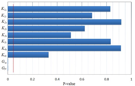
F-test is applied to evaluate the P-value of factors relative to the DOE response, and the threshold of significance is used as $P_0=$0.05. The P-values of the 10 factors are presented in Fig. 8. As can be seen, the two factors $G_{xz}$ and $G_{yz}$ have a lower P-value than the threshold, so they are taken as input variables of Kriging model for model updating.

Fig. 8P-value of all factors of example 2

The Kriging model can be constructed based on the 150 sampling points, the basic parameters ${\theta }_{xz}$ and ${\theta }_{yz}$ are solved as: ${\theta }_{xz}=$ 40.0477, ${\theta }_{yz}=$ 12.9745, which correspond to the input variables $G_{xz}$ and $G_{yz}$ respectively.

10 checking points are generated and used to assess the accuracy of the Kriging model. The output response at each checking points of Kriging model and analytical model are shown as Fig. 9. The RMSE is evaluated as about 4.2 %, which means the constructed Kriging model has an acceptable accuracy.

Fig. 9The response values of checking points of example 2

5.2.2. Model updating results and discussion of example 2

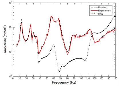
Based on the constructed Kriging model, the optimization process is operated within the same variables scope as DOE level shown as Table 6. After 1000 iterations by MIGA, the updated results of the two selected parameters are obtained: $G_{xz}=$0.1636, $G_{xz}=$0.2244. Then the initial analytical model is modified by using the two updated parameters and the rest 8 parameters keeping their initial values. The three AFRF curves (in $Z$ directional) at $P_1$ are plotted in Fig. 10, they are updated curve, noise contaminated experimental curve and initial analytical curve respectively. The updated curve agrees well with the experimental curve, and the residual error nearby 80 Hz may because the random noise effect is locally strengthened.

Fig. 10Comparison between initial AFRF curve and updated AFRF curve of example 2

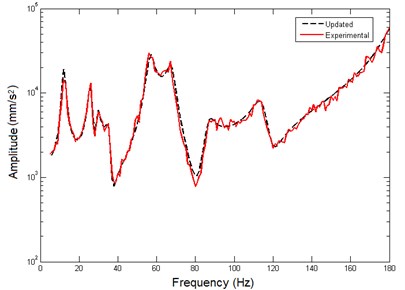
In order to further verify the prediction capability of the analytical model after model updating, another two AFRF cures at prediction position $P_2$ are extracted in $Y$ direction and $Z$ direction DOF respectively that plotted in Fig. 11, which presents a good agreement between the two curves. Moreover, the analysis frequency band is extended to 180 Hz at $P_1$, both the updated curve and the experimental curve are plotted in Fig. 12. Again, the two curves can coincide well in the extended 30 Hz frequency range. It can be considered that the analytical model has a good prediction capability.

This can be concluded that the analytical model and experimental model have almost the same behavior of FRF, and the analytical model is updated successfully by using FRF data.

Fig. 11Comparison between AFRF curves at P2

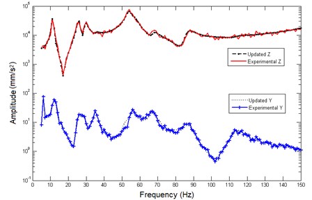
Fig. 12Comparison between AFRF curves of extended frequency band at P1

6. Conclusions

In this paper, Kriging model is introduced into the FRF based model updating. A method is proposed to the model updating examples of honeycomb structure and solar array structure by using AFRF data. Their Kriging models are constructed based on the input variables respectively, which are selected successfully by F-test method based on the DOE results which generated based on the sampling method of Optimal Latin Hypercube. The Kriging model can replace the FEA with acceptable accuracy assessed by RSME criterion, and the MIGA is an appropriate algorithm for the optimization problem of model updating.

Though the Kriging model is constructed by a fraction number of the initial input variables, the results of model updating can achieve a good agreement between the AFRF curves of analytical model and experimental model, even when the measured data of experimental AFRF is contaminated by noise. It turns out that Kriging method is an effective technique for FRF based model updating, and future studies could investigate the FRF based data of physical structure to validate its conviction.