Algorithm for noise reduction for strongly contaminated chaotic oscillators based on the local projection approach and 2D wavelet filtering

1. Introduction

The task of noise reduction is a central theme in a wide variety of fields. Chaotic time series have inherently broad spectra and are not amenable to conventional spectral noise filtering, since linear filters severely distort even clean chaotic signals. Over the past two decades, a number of important algorithms have been developed for noise reduction of chaotic signals. A comprehensive overview of these algorithms can be found in [1, 2]. All noise reduction methods for chaotic time series may be classified as model-based or model-free. While model-based reduction can be applied for systems with known analytical models, model-free noise reduction provides a superior alternative for experimental data. Two of the major model-free noise reduction techniques are chaos-based smoothing [3] and wavelet thresholding [4, 5]. While details of chaos-based methods vary, they share a common fundamental element: they approximate the local chaotic dynamics in the neighbourhood (of size $\epsilon$) of a reference point (here the appropriate neighbours mean that the wave forms of the data segments covered by the neighbours are well matched to those of the reference phase point). When noise is weak, the chosen value of ε can be small, and the approximation to the local dynamics can be quite accurate. When the noise is strong, however, the accuracy of the neighbourhood is degraded, the chance of picking a false neighbour is increased, and the local chaotic dynamics cannot be accurately estimated [2]. The over-embedding technique with a time delay $\tau =\text{1}$ and an appropriately longer embedding window contribute to the determination of valid neighbours at strong noise [6], but the nearest neighbouring vectors identified in this way inevitably differ due to sensitivity to the initial conditions according to the Lyapunov exponents. Because the local projection (LP) approach decomposes the reconstructed phase space into two orthogonal subspaces (i.e. the signal subspace and the noise subspace) based on linear combinations of the columns of the neighbourhood array, over-embedding with a too long embedding window leads to distortion of even clean chaotic signals. Of course, this limitation arises due to the nature of chaotic signals, and cannot be avoided in cases where the neighbours are considered as strands of several consecutive vectors of reconstructed phase-space rather than separate vectors [7, 8]. On the other hand, wavelet shrinkage methods require an opportune selection of parameters or some “a priori” knowledge of the system or the noise mechanisms. These drawbacks motivate the search for new methods that can efficiently recover continuous-time chaotic signals in heavy-noise environments [2].

In this paper, the advantages of both chaos-based and wavelet shrinkage methods have been combined. Namely, the necessary threshold for wavelet shrinkage is calculated by estimating the noise subspace of the neighbourhood of the reference points using proper orthogonal decomposition, and two-dimensional (2D) discrete stationary wavelet transform (SWT)-based filtering is performed on the neighbourhood. As demonstrated later, this action allows better recovery of the signal of the underlying chaotic dynamics at low signal-to-noise-ratio (SNR), not only reducing noise.

2. Description of the algorithm

Let $x_i=s_i+w_i$ denote the time series contaminated by additive noise, where $s_i$ are the clean data generated by a dynamical system and $w_i$ is the additive noise. For a time series ${\left\{x_i\right\}}_{i=1}^L$ with $L$ samples, the phase points can be reconstructed by time delay embedding [3], i.e., ${\left\{{\mathbf{x}}_i\right\}}_{i=1}^{L-\left(d-1\right)\tau }$:

where $d$ is the embedding dimension, $\tau$ is the time delay, and ${\left(\bullet \right)}^T$ denotes the transpose of a real matrix. Over-embedding with the time delay $\tau =\text{1}$ is used and the embedding dimension is defined arbitrarily as approximately equal to two cycles of the attractor. Usually, the near neighbourhood of the reference point ${\mathbf{x}}_i$ is defined as:

where $\epsilon$ is the size of the neighbourhood. Because defining the size of the neighbourhood ${\mathbf{N}}_i$ at strong noise is problematic, a given number $K$ of nearest neighbours is found, rather than a neighbourhood of fixed radius. The phase vectors of the neighborhoods are rearranged in such a way that the reference point ${\mathbf{x}}_i$ would be in the centre of the neighborhoods array and the nearest neighbours in ascending order of the Euclidean distance from the reference point ${\mathbf{x}}_i$. Assuming that the noise is white and Gaussian, the local phase space, i.e., the neighbourhood ${\mathbf{N}}_i$ of the reference point ${\mathbf{x}}_i$, can be divided into an $M$-dimensional signal subspace and a $\left(d-M\right)$ –dimensional noise subspace, where $M$ is the minimum embedding dimension of the dynamical system [6, 9, 10]. The signal subspace contains most of the clean signal plus a certain amount of the noise components, while the noise subspace contains most of the noise components and a certain, small, amount of the signal components. For a preset $M$, the noise subspace can be estimated by performing the standard singular value decomposition (SVD) ${\mathbf{R}}_i=\mathbf{U}\mathbf{\Lambda }{\mathbf{V}}^T$ for the covariance matrix ${\mathbf{R}}_i=(1/K-1){\tilde{\mathbf{N}}}_i{\tilde{\mathbf{N}}}_i^T$ of the zero-mean neighbourhood ${\tilde{\mathbf{N}}}_i$, i.e., ${\tilde{\mathbf{N}}}_i={\mathbf{N}}_i-{\stackrel{-}{\mathbf{N}}}_i$, where ${\stackrel{-}{\mathbf{N}}}_i$ is the column matrix of the mean over dimensions $1$,…, $d$. Sorting the eigenvalues $\mathbf{\Lambda }=\mathrm{d}\mathrm{i}\mathrm{a}\mathrm{g}\left({\lambda }_1,{\lambda }_2,\dots ,{\lambda }_d\right)$ in descending order, the eigenvectors ${\mathbf{U}}_s=\left[{\mathbf{u}}_1,\dots ,{\mathbf{u}}_M\right]$, associated with the $M$ largest eigenvalues, span the signal subspace, and the eigenvectors ${\mathbf{U}}_n=\left[{\mathbf{u}}_{M+1},\dots ,{\mathbf{u}}_d\right]$, corresponding to the $\left(d-M\right)$ smallest eigenvalues, span the noise subspace, respectively. Then the noise part of neighbourhood ${\mathbf{N}}_{in}$ can be estimated by projecting ${\tilde{\mathbf{N}}}_i$ into noise subspace, i.e., ${{\mathbf{N}}_{in}=\mathbf{U}}_n{\mathbf{U}}_n^T{\tilde{\mathbf{N}}}_i$.

Finally, the neighbourhood ${\mathbf{N}}_i$ is denoised by employing a 2D SWT-based filter and using the estimated noise level for wavelet coefficients thresholding. The 2D dyadic discrete SWT enables to capture the common shape of the phase vectors of neighborhoods. The steps of the final stage of the proposed algorithm are as follows:

1) 2D signal of pure noise ${\mathbf{N}}_{in}$ is decomposed by 2D multilevel SWT into its approximation coefficients matrix ${\mathbf{A}}_{in}$ and detail coefficients matrices ${\mathbf{D}}_{inj}^c$ of decomposition level $j$, where index $c$ denotes the horizontal, vertical and diagonal detail coefficients. The threshold value $t_{ij}^c$ at decomposition level $j$ is defined as the 0.99 quantile of coefficients ${\mathbf{D}}_{inj}^c$.

2) Analogous decomposition into its approximation coefficients matrix ${\mathbf{A}}_i$ and detail coefficients matrices ${\mathbf{D}}_{ij}^c$ is performed on the 2D noisy signal (neighbourhood) ${\mathbf{N}}_i$ and the coefficients ${\mathbf{D}}_{ij}^c$ are adjusted at each decomposition level via soft thresholding using the estimated threshold values $t_{ij}^c$. The thresholding of the wavelet coefficients is usually applied only to the detail coefficients rather than to the approximation coefficients, since the latter represent “low-frequency” terms that usually contain important components of the signal, and are less affected by the noise [4].

3) Applying the inverse SWT to the threshold wavelet coefficients, the estimate ${\widehat{\mathbf{N}}}_i$ is obtained, which approximates the neighbourhood of the noise-free vector time series and the central column of the filtered neighbourhood ${\widehat{\mathbf{N}}}_i$ denotes the filtered $i$th phase point.

4) The steps of filtering are repeated for all phase points.

As each element of the time series ${\left\{x_i\right\}}_{i=1}^L$ occurs as an entry of one of $d$ successive phase vectors ${\mathbf{x}}_k$, $k=n-\left(d-1\right)\tau ,\dots ,n$, there are $d$ enhanced entries that may be different in value [6, 11]. The time-aligned weighted average using the Hamming window as a weighted average transformation over these values is taken as the enhanced element ${\widehat{s}}_n$. This process corresponds to a suppression the distortion of the elements in both ends of the phase point, emphasizing the time-centred value of each projected point.

3. Results

First of all, the proposed method was tested on two numerical examples: the $x$ component of the chaotic Rössler system and the nonlinear Duffing oscillator, which is known to describe many important oscillating phenomena in some nonlinear physical and engineering systems. The Rössler attractor is governed by the following system of equations:

Here we used $a=\text{0.398}$, $b=\text{2.0}$, and $c=\text{4}$. A time series was generated using the ODE45 integrator in Matlab. The solution was sampled at time intervals $\delta t=\text{0.1}$ (with a main oscillation period of approximately 67 samples) and 2000 samples, after the first 200 samples were discarded, were adopted for analysis. The nonlinear Duffing oscillator is governed by the following system of equations:

Here we used $\delta =\text{0.5}$, $\gamma =\text{0.37}$, and $\omega =\text{1.0}$. A time series was generated using the ODE45 integrator in Matlab, and the solution was sampled at time intervals $\delta t=\text{0.1}$. All the signals were contaminated with additive white Gaussian noise at various signal-to-noise ratios (SNRs).

The level of the decomposition $j=\text{3}$ and biorthogonal wavelet bior2.2 for the two-dimensional discrete SWT were chosen. For the SWT, if a decomposition at level $j$ is needed, $2^j$ must divide $size({\mathbf{N}}_i,1)$ and $size\left({\mathbf{N}}_i,2\right)$. Therefore, in this paper we set the embedding dimension $d=\text{128}$ and time delay $\tau =\text{1}$, and the first 16 nearest neighbours are used for each reference phase point.

The performance of the denoising process was quantified in terms of SNR improvement (SNRimp) in decibels (dB), and root mean square error (RMSE) defined as follows:

where $L$ is the signal length in samples, $s\left(n\right)$ is the noise-free signal, $x\left(n\right)$ is the observed noisy signal, and $\widehat{s}\left(n\right)$ is the filtered signal. The performance of the algorithm was evaluated by means of a 20-trial Monte Carlo simulation whereby the signals are contaminated by various realizations of additive zero mean white Gaussian noise at a SNR from 20 to 0 dB. All data processing and analyses were performed with MATLAB software (version R2007b, The MathWorks, Natick, MA).

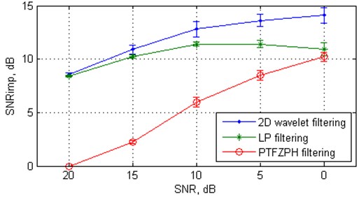
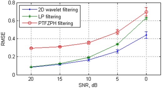
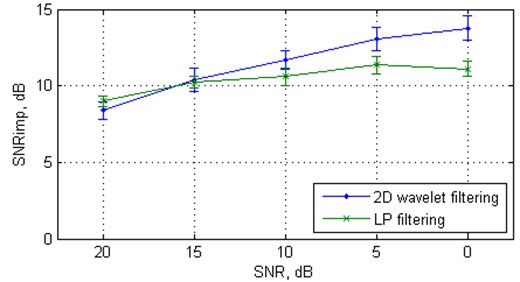
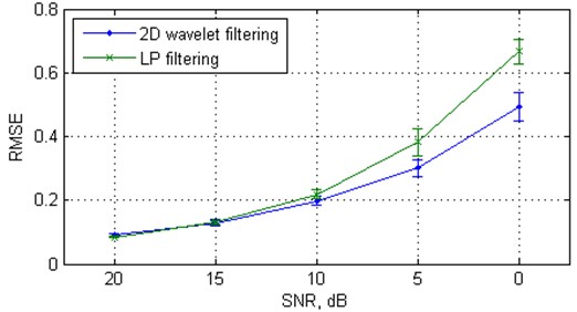
To appreciate the effectiveness of the proposed algorithm, we first compare its denoising performance with the nearest state-of-the-art approach – classical local subspace method and recently introduced parallel-type fractional zero-phase (PTFZPH) method [12]. It is worth noting that the parameters of the reconstructed phase space (viz. embedding dimension, time delay) and the size of the neighbourhood for both proposed and LP method were defined as identical. The variations of the mean SNRimp values from 20 independent Monte Carlo trials with SNR for these methods applied to the Rössler signal are shown in Fig. 1(a) and the variations of the mean RMSE values are shown in Fig. 1(b). Clearly, the parallel-type fractional zero-phase method leads to the largest distortion of the filtered signal in comparison with the other two methods. Therefore, it is not analyzed hereafter. From Fig. 1, we can see that the proposed algorithm outperforms the local subspace approach at low SNR: from 15 to 0 dB. For example, the proposed algorithm provides about 14.11 dB, on average, improvement in SNRs at SNR = 0 dB, while the classical local subspace approach-based algorithm manages only 10.92 dB of improvement. Similar results are obtained for Duffing oscillator (Fig. 2).

Fig. 1The mean values and standard deviations (with error bars) of the SNRimp and RMSE from 20 independent Monte Carlo trials versus white Gaussian noise level for the Rössler signal

a) SNRimp

b) RMSE

While the SNRimp and RMSE are convenient metrics to quantify the quality of denoising, for a chaotic signal it is important to examine how much the invariant parameters of the underlying nonlinear dynamics such as fractal dimensions, entropies, or Lyapunov exponents, are recovered after denoising. Therefore, we have used for our study two algorithms namely modified 0-1 test and the largest Lyapunov exponent (LLE) for experimental chaos detection in the filtered time series. The 0-1 test [13] is a binary test for chaos detection which does not require any prior knowledge on the equations of the underlying systems. The distinction between regular and chaotic dynamics is extremely clear by means of a diagnostic variable, which has values close to zero for regular orbits and close to one for the chaotic orbits. The test has been successfully applied to continuous time systems, discrete time systems, integer-order systems as well as fractional-order systems [14]. As the use of binary 0-1 test in his first version for chaos detection is limited to detect chaos in oversampled time series observations, a modified 0-1 test is proposed [15], in which, binary 0-1 test is applied to the discrete map of local maxima and minima of the original observable in contrast to the direct observable. In our experiment, the scores of the 0-1 test applied to the filtered Rössler and Duffing signals were in the range of 0.97-0.99 for both proposed and LP denoising algorithms, i.e., detect the dynamics as chaotic, and as results, cannot capture the subtle difference between signals filtered by proposed and LP algorithms. The largest Lyapunov exponent (LLE) in this case appears to be more appropriate for detecting small changes in the dynamics. LLE of the denoised Rössler and Duffing signals was examined, using the algorithm of Rosenstein [16] because of its advantages. The Rosenstein algorithm is fast, easy to implement, and robust to changes in the following quantities: embedding dimension, size of data set, reconstruction delay, and, relatively, noise level. The LLE was calculated using the embedding dimension $d=\text{5}$ and time delay $\tau =\text{6}$.

Fig. 2The mean values and standard deviations (with error bars) of the SNRimp and RMSE from 20 independent Monte Carlo trials versus white Gaussian noise level for the Duffing oscillator

a) SNRimp

b) RMSE

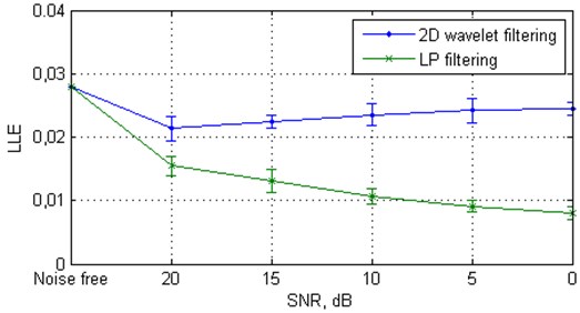
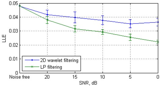
Fig. 3 shows the variation of LLE dependent on SNR for the signal denoised by the proposed algorithm and for the signal denoised by the LP algorithm. In the first case one can see that the LLE decreases with respect to the noise-free case, but remains approximately constant and clearly positive over SNR scales, indicating chaotic underlying dynamics, whereas in the second case, the LLE quickly tends to zero.

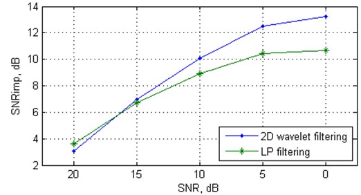
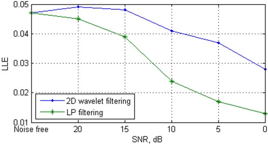
In order to evaluate the effectiveness of the proposed algorithm in real world applications, we have applied the algorithm to a human breath time series. It is known [17], that human respiration demonstrates chaotic behaviour. The respiratory signals are taken from the combined measurement of ECG, Breathing and Seismocardiograms Database (cebsdb) (http://physionet.org/physiobank/database/cebsdb/). The clean respiratory signal (from record, numbered b001) with length of 30 fundamental frequency periods was downsampled to about 60 samples per period. Fig. 4(a) shows the SNRimp values and Fig. 4(b) shows the variation of LLE dependent on SNR for the respiratory signal denoised by the proposed algorithm and for the signal denoised by the LP algorithm. As in the case of synthetic signals, the performance of the proposed algorithm is superior to the nearest state-of-the-art LP method.

Fig. 3Largest Lyapunov exponent from 20 independent Monte Carlo trials versus white Gaussian noise level for the clean and filtered Rössler data, the clean and filtered Duffing data

a) The clean and filtered Rössler data

b) The clean and filtered Duffing data

4. Conclusion

An adaptive strong noise reduction approach based on the over-embedding method for phase space reconstruction and applying a 2D SWT-based filter for neighbourhood array denoising was proposed in this paper. The noise reduction experiment on the noisy Rössler signal, Duffing oscillator, and a real-world signal (respiratory time series) showed that the proposed approach is more effective in removing strong white Gaussian noise, and preserving the characteristics of the underlying nonlinear dynamics, than the routine LP algorithm for continuously sampled noisy time series. The image-oriented filter based on the 2D dyadic discrete SWT enables the capturing of the common shape of the neighborhoods, and also preserves the individual properties of the phase vectors better than LP approach based on linear combinations of the orthogonal components of the neighborhoods. This was demonstrated using convenient metrics to quantify the quality of denoising, i.e., SNRimp, RMSE, and invariants, to characterize deterministic chaos, i.e., LLE. The relative limitation of the proposed algorithm (which is common to all nearest neighbors algorithms) is the excessive amount of computation.

Fig. 4The values of the SNRimp and Largest Lyapunov exponent versus white Gaussian noise level for the respiratory signal

a) SNRimp

b) Largest Lyapunov exponent