Synthesis of running RMS-induced non-Gaussian random vibration based on Weibull distribution

1. Introduction

Random vibration testing is usually used to bring a test item to failure to identify weaknesses in the product or to verify if the product can survive a particular random vibration environment. Random vibration controllers accomplish this goal by producing a power spectral density (PSD) that would expose the test item to the type of vibratory environment that the test item would experience in a real-world setting. Since PSD does not contain phase information, vibration controllers always assume the phase of each frequency component follows a 0 to 2$\pi$ uniform distribution when producing time history using the PSD. This leads to data with Gaussian distribution. Non-Gaussian vibration is usually encountered, especially in the road transportation. W. H. Connon and D. Charles points out that when vehicles are running on irregular roads, the random excitation placed on vehicles is often non-Gaussian. The tail of measured acceleration PDF is wider and the middle is sharper when compared with Gaussian distribution [1, 2]. This difference may lead to totally different accumulated fatigue damage, because most fatigue damage is caused by 2 to 4$\sigma$ [3]. When peak value exceeds 3$\sigma$, products fail quickly. MIL-STD810 points out that we should always check if the field tested data is non-Gaussian and the testing hardware and software is appropriate [4]. The time waveform replication (TWR) is frequently referred to as a methodology for non-Gaussian testing. The basic idea of TWR is to reproduce a sequence of instantaneous values of the vibration process. Such a test may be non-Gaussian, however this is only a replication of one particular measured record, not a simulation of a specified road type. Besides, MIL-STD810F says that TWR is usually used for controlling transient signals or short time lasting random vibration [4]. With these drawbacks of TWR, many researchers presented some other methods to simulate non-Gaussian vibration. Smallwood used three zero-memory nonlinear (ZMNL) functions to transform Gaussian vibration to non-Gaussian vibration [5, 6]. These functions all give similar, but not identical results. Each covers similar but slightly different ranges of skewness and kurtosis. Each will result in slightly different distributions. Initially, this method was recommended in the form where non-Gaussian time histories are first prepared offline before running a test and, then, these time histories are reproduced on the shaker in the Time Waveform Replication mode. It was only later when this method was extended and modified into a method that can be used in the closed-loop frequency domain control mode [8, 9]. This method is easy to implement but it significantly reduces the controller’s dynamic range compared to the traditional Gaussian random testing and may disrupt the PSD shape. Stein wolf developed a special phase selection method [7-9]. The essence of this method is that the amplitudes are still responsible for the PSD, whereas the phases are not all random as they were in the classic IFFT generation. Instead, some of the phases are now used to adjust kurtosis. Thus, both characteristics, the PSD and the kurtosis, are controlled independently of each other. Rouillard et al. presented a novel technique by which non-Gaussian vibrations are synthesized by generating a sequence of random Gaussian processes of varying RMS levels and durations [10-15]. John et al. studied the relationship between kurtosis and fatigue damage spectrum (FDS) [16]. He declares that the fatigue damage spectrum shows the increasing fatigue damage across all frequencies that accompany the increased kurtosis levels that cause the faster product failure.

To synthesize the non-Gaussian random vibration, both the PDF and the damage effects must be considered. A new method is presented in this paper to synthesize the non-Gaussian random vibration that is characterized by the running RMS (root mean square). The essential idea is to model the non-Gaussian signal by a Gaussian signal multiplied by a slowly varying amplitude modulation function (AMF). A two-parameter Weibull distribution is used to model the PDF of the running RMS and to create the AMF. The shock response spectrum (SRS) is used to detect significant shocks within the non-Gaussian field signal. No sequence of random Gaussian processes of varying RMS levels and durations needs to be generated in this method, which makes it much easier to be implemented than that Rouillard et al. used [10-15]. A case study is presented to show that the synthesized non-Gaussian signal has the same PSD, kurtosis, PDF and FDS as the field data.

2. Theory

2.3. Fatigue damage spectrum and shock response spectrum

All structures experience fatigue as they are repeatedly exposed to adequate levels of stress. The total damage a product experiences in a particular time period can be calculated from field data and plotted for a specific range of frequencies. The FDS is essentially a plot that shows the responses of a number of single degree of freedom (SDOF) systems to a base input acceleration time history. Many SDOF systems tuned to a range of natural frequencies are assessed using the same input. The final plot, the FDS, shows the fatigue damage encountered for a particular SDOF system anywhere within the analyzed time, as shown in Fig. 1 and Fig. 2.

Fig. 1SDOF systems for calculation of FDS

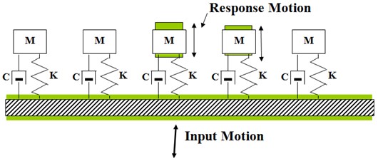
Fig. 2Calculation procedure of the FDS

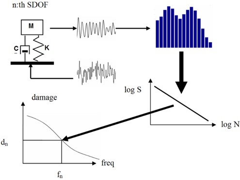
For a SDOF system with a natural frequency $f_n$ and a damping ratio $\xi$, the output relative displacement $x_d$ to an input acceleration $x_a$ can be calculated using a ramp invariant digital filter method [22]. With the output $x_d$, the cumulative damage can be calculated in both time domain and frequency domain. In time domain, RFCC method is usually used to count cyclic numbers at different stress levels. Then S-N curve [23] and Miner’s rule [24] are combined to calculate fatigue damage:

12

$N_i=c{S}_i^{-b},$

13

$D_t=\sum _{i=1}^p\frac{n_i}{N_i}=\sum _{i=1}^p\frac{n_i{S}_i^b}{c},$

where $n_i$ is the number of cycles exposure at $S_i$ ($i=\text{1, 2,...,}p$). $p$ is the number of stress levels considered. $N_i$ is fatigue life at stress $S_i$, $b$ is the fatigue exponent, $D_t$ is the total damage index calculated in time domain.

The stress is assumed to be proportional to relative displacement [25]:

14

$S=k{x}_d.$

The total damage can be calculated as:

15

$D_t=\sum _{i=1}^p\frac{n_i}{N_i}=\sum _{i=1}^p\frac{n_i{k}^b{x}_{d,i}^b}{c}=\frac{k^b}{c}\sum _{i=1}^p{n}_i{x}_{d,i}^b.$

In frequency domain, Rayleigh distribution of response stress maxima is assumed and used to calculate the stress cycles [26]:

16

$p\left(S\right)=\frac{S}{{\sigma }_S^2}{e}^{\frac{-S^2}{2{\sigma }_S^2}},$

where $S$ is the stress value of peaks, ${\sigma }_S$ is the RMS of the stress time history.

The total damage can be calculated as:

17

$D_f=n_p^{+}T\underset{0}{\overset{+\mathrm{\infty }}{\int }}\frac{p\left(S\right)}{N\left(S\right)}dS=\frac{n_p^{+}T}{c}\underset{0}{\overset{+\mathrm{\infty }}{\int }}p\left(S\right)S^{b}dS=\frac{f_{n}T}{c}\underset{0}{\overset{+\mathrm{\infty }}{\int }}p\left(S\right)S^{b}dS,$

where $n_p^{+}$ can be replaced by the natural frequency $f_n$ for a lightly damped SDOF system response, $T$ is the total time of exposure to the stress environment.

Solving Eq. (17) with Eq. (16) leads to:

18

$D_f=\frac{f_{n}T}{c}{\left(2{\sigma }_{{\mathrm{}}_S}^2\right)}^{\frac{b}{2}}\mathrm{\Gamma }\left(1+\frac{b}{2}\right)=\frac{f_{n}T}{c}{k}^b{\left(2{\sigma }_{{\mathrm{}}_d}^2\right)}^{\frac{b}{2}}\mathrm{\Gamma }\left(1+\frac{b}{2}\right),$

where $\mathrm{\Gamma }$ is the Gamma function, ${\sigma }_d$ is the RMS of relative displacement.

The RMS of relative displacement can be calculated using:

19

${\sigma }_d=\sqrt{{\int }_{f=f_{low}}^{f=f_{hi}}\left({\left|H\left(f\right)\right|}^2{G}_{xx}\left(f\right)\right)df},$

where $H\left(f\right)$ is the transmissibility of a SDOF system with a natural frequency of $f_n$ and a damping ratio of $\xi$.

Since different kurtosis leads to different number of peak accelerations in the test, and these peak accelerations are primarily responsible for damage that a product experiences in the field, the FDS should show the difference when calculated for Gaussian and non-Gaussian vibrations.

The effects of the shock loads are generally depicted in a SRS. Like the FDS, the SRS is essentially a plot that shows the responses of a number of SDOF systems to a base input acceleration time history, as shown in Fig. 1. The only difference is that the SRS is generated by calculating the maximum response of a SDOF system to the input. The final plot, the SRS, shows the largest response encountered for a particular SDOF system anywhere within the analyzed time.

Since the essential idea of the new synthesis method is to model the non-Gaussian signal by a Gaussian signal multiplied by an AMF:

20

$x_{nonGaussian}=x_{Gaussian}{f}_{AMF},$

significant shocks in the field data must be first identified and separated. To detect if there are significant shocks in the field data, the response of a number of SDOF systems to the field data is firstly calculated in time domain. Then the response is divided into $M$ consecutive segments and the maximum value is calculated for each segment. Finally the ratio between this maximum value and the SRS computed from the PSD, which is calculated from the whole time history using Welch method, is used to show where the significant shock is:

21

$R_{n,i}=20\mathrm{l}\mathrm{g}\frac{y_{n,i}}{SR{S}_n},\mathrm{}\mathrm{}\mathrm{}\mathrm{}n=1,\mathrm{}2,...,N,\mathrm{}\mathrm{}\mathrm{}\mathrm{}i=1,\mathrm{}2,...,M,$

where $y_{n,i}$ indicates the maximum value calculated for the $i$th segment and the $n$th SDOF system, $SR{S}_n$ indicates the SRS calculated form PSD for the $n$th SDOF system.

3. Synthesis method

A new method is presented to synthesize the non-Gaussian random vibration characterized by the running RMS. The procedure uses three phases to streamline the process:

Phase 1: Check the characteristics of measured vibration signal.

1. Obtain the environment acceleration time history, resample if needed.

2. Calculate the kurtosis of measured signal to see if it is Non-Gaussian or not.

3. Calculate the PSD of measured signal using Welch’s method.

4. Use SRS to detect significant shocks (see Eq. (21)).

Phase 2: synthesize the Non-Gaussian random vibration.

1. Create the stationary Gaussian signal using the PSD calculated in step 3, Phase 1.

2. Calculate the probability distribution function $F_{RMS}$ of the running RMS of the field data.

3. Use a two parameter Weibull distribution to model the probability distribution of the running RMS.

The cumulative distribution function of Weibull distribution can be expressed as:

where $x$ is the random variable, $L$ is the scale parameter, $K$ is the shape parameter.

To find the correct $L$ and $K$, the probability distribution function of the assumed Weibull distribution $F_{Weibull}$ and the running RMS $F_{RMS}$ are used to form an objective function using least squares method:

where $x$ are the values of the running RMS, depending on how many bins are used to calculated the probability distribution function of the running RMS, $i$ indicates the $i$th iteration, $std$ indicates standard deviation. Note that both $F_{RMS}$ and $F_{Weibull}$ are vectors.

The MATLAB function “fminsearch” is used find the right $L$ and $K$, so that the standard deviation of error between these two probability distribution functions is minimized.

1. Use the determined $L$ and $K$ to create the AMF and to get the required Non-Gaussian signal.

2. To create the appropriate AMF, the kurtosis of the field data is used as an objective value. The AMF is created from the Weibull distribution function and multiplied with the Gaussian signal created in step 1, Phase 2, to get the synthesized signal. Compare the kurtosis of the synthesized signal with the objective value. Do iterations until the objective value is reached. The synthesized non-Gaussian signal is scaled to have the same RMS as the field data.

Phase 3: compare the characteristics of the synthesized Non-Gaussian signal and the field data.

1. Compare the PSD.

2. Compare the PDF.

3. Compare the fatigue, e.g., cyclic numbers and FDS.

4. Case study

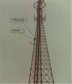
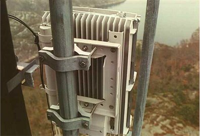
In this case study, a new method for synthesizing the non-Gaussian random vibration is developed and examined by the field data. The field data provided by Prof. Kjell Ahlin is from an Ericsson Mast Project and is shown in Fig. 3. The test item and setup are shown in Fig. 4.

Fig. 3Field data

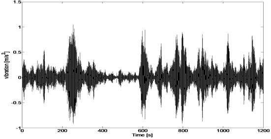
Fig. 4Test item and setup

This is a non-Gaussian signal with kurtosis equals to 9.4262. Eq. (21) is used to detect significant shocks (see Fig. 5). The ratio is shown in the third dimension by the color. As we can see from Fig. 5, there are only some insignificant shocks superimposed on the underlying random vibration signal.

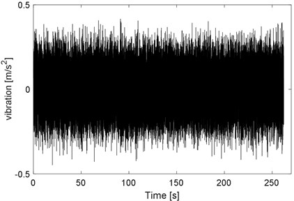
The PSD of the field data is calculated using Welch method with 4096 points hanging window and 50 % overlapping. Gaussian signal is generated using the same but smoothed PSD and is shown in Fig. 6.

Fig. 5Detection of shocks

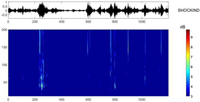
Fig. 6Synthesized Gaussian signal using the same PSD calculated from field data

The PSD and PDF of both the field data and the synthesized Gaussian signal are shown in Fig. 7 and Fig. 8. As we can see, the PDF of the field data is obviously different from that of the synthesized Gaussian signal, although the PSD are basically the same.

Fig. 7PSD of field data and synthesized Gaussian signal

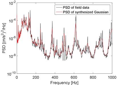
Fig. 8PDF of the field data and the synthesized Gaussian signal

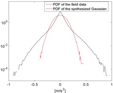
Fig. 9The running RMS

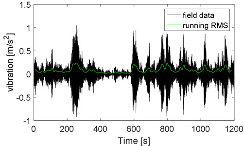
Fig. 10PDF of the running RMS using different number of bins and Rayleigh distribution

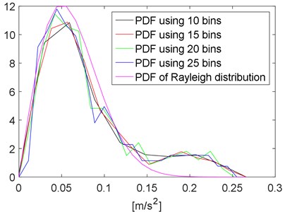
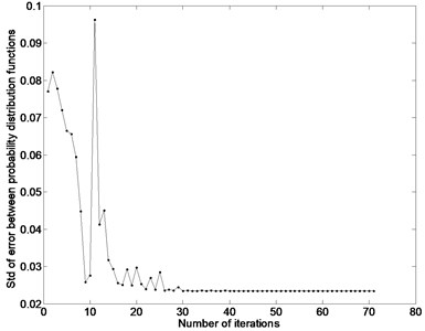
Fig. 11The iteration to determine L and K

The running RMS and its PDF using different number of bins are calculated and shown in Fig. 9 and Fig. 10. The running RMS is calculated using 10 s frames with 50 % overlapping. From Fig. 10 we can see that, despite of the numbers of bins, the PDF of the running RMS is similar to the PDF of a given Rayleigh distribution. To be more general, a two-parameter Weibull distribution is used to model the probability distribution function of the running RMS Eq. (22).

Iteration method described in Section 3 (step 3, phase 2) is used to determine $L$ and $K$. The iteration process is shown in Fig. 11. The probability distribution function of resulted Weibull distribution is shown in Fig. 12, together with the probability distribution function of the running RMS.

As the parameters of the Weibull distribution are determined, the AMF can be created and the non-Gaussian signal can be synthesized using the iteration method presented in Section 3 (step 4, phase 2). The synthesized non-Gaussian signal is shown in Fig. 13, together with the field data (the time duration of the synthesized non-Gaussian signal is adjustable). Note that some care must be taken to have the time scale for the AMF selected properly, since inappropriate selection of time scale may lead to inaccurate PDF and/or PSD.

The PSD and PDF of the field data and the synthesized non-Gaussian signal are very similar (see Fig. 14 and 15), which proves the effectiveness of the new method.

For comparison, the cycle counting with the RFCC and Dirlik method can be performed directly on the field data (acceleration signal), the synthesized Gaussian signal and non-Gaussian signal. The results are shown in Fig. 16. As we can see, the Dirlik method is equivalent to the RFCC for Gaussian signal. Big error can be introduced by the Dirlik method for non-Gaussian signal. The RFCC results for the field data and synthesized non-Gaussian signal are very similar.

Fig. 12The probability distribution function of the running RMS and Weibull distribution

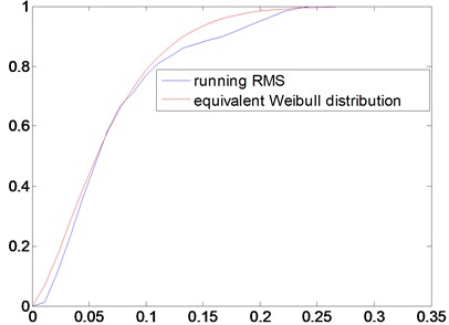
Fig. 13Field data and synthesized non-Gaussian signal

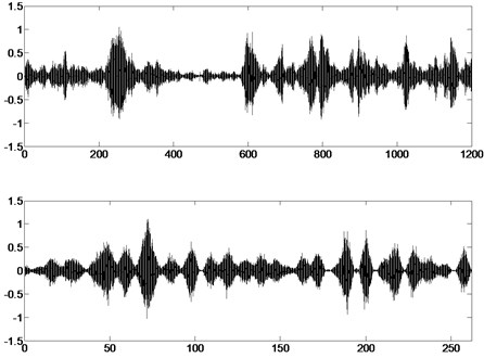
Fig. 14Mast vibration signal power spectral density. The PSD of the field data and the synthesized non-Gaussian signal

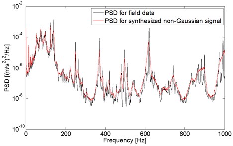
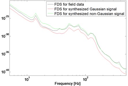
Fig. 17 shows the FDS calculated for the field data, the synthesized Gaussian and non-Gaussian signal in the time domain using Eq. (15). For comparison, $k$ and $c$ are normalized to 1. From Fig. 17 we can see that the FDS of the field data and the synthesized non-Gaussian signal are very similar. This again proves the effectiveness of the new method. Besides, we can also see that larger kurtosis leads to larger fatigue damage.

Fig. 15Amplitude probability density. PDF for field data and synthesized Gaussian and non-Gaussian signal

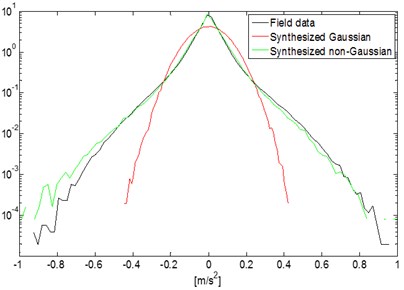
Fig. 16Number of cycles versus data ranges for RFCC and Dirlik

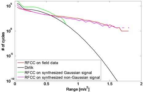
Fig. 17Fatigue damage spectrum. The FDS of the field data, synthesized Gaussian and non-Gaussian signal

5. Conclusion

A new method for synthesizing the running RMS-induced non-Gaussian Random Vibration is developed and examined by field data. Conclusions are as below:

1. This method is limited to the case of the running RMS-induced non-Gaussian signals, which contain no significant shocks.

2. The synthesized non-Gaussian signal has the same PSD, kurtosis, PDF and FDS with the field data, which proves the effectiveness of the new method.

3. The Dirlik methods are equivalent to the RFCC method for Gaussian signal and can introduce big error for non-Gaussian signal.

4. Larger kurtosis leads to larger fatigue damage.

5. Weibull distribution can be used to simulate the statistical distribution of the running RMS and to synthesize the running RMS-induced non-Gaussian signal.