Abstract
Aiming at the problems existing in previous chaos time series prediction methods, a novel chaos times series prediction method, which applies modified GM(1, 1) model with optimizing parameters to study evolution laws of phase point L1 norm in reconstructed phase space, is proposed in this paper. Phase space reconstruction theory is used to reconstruct the unobserved phase space for chaotic time series by C-C method, and L1 norm series of phase points can be obtained in the reconstructed phase space. The modified GM(1, 1) model, which is improved by optimizing background value and optimizing original condition, is used to study the change law of phase point L1 norm for forecasting. The measured data from stabilized platform experiment and three traditional chaos time series are applied to evaluate the performance of the proposed model. To test the prediction method, three accuracy evaluation standards are employed here. The empirical results of stabilized platform are encouraging and indicate that the newly proposed method is excellent in prediction of chaos time series of chaos systems.
1. Introduction
Prediction is an inferring procedure about the future unknown states using some certain methods or techniques based on system historical and current known states. Time series forecasting is one of the most important quantitative models in which historical observations of the same variable are collected and analyzed to develop a model that captures the underlying data generating process [1]. Among the different types of time series, chaotic time series can be commonly found in natural phenomena [2]. Among the prediction methods, Grey System Theory, pioneered by Deng (1982), is a new method for studying uncertain problems with less data and poor information, and is applicable to system analysis, data processing, modeling, prediction, decision making and control [3]. GM(1, 1) model is the most frequently used model in grey predictions which is suitable for the observed data with exponential distributing, and it has been widely and successfully applied to various systems such as financial, economic, scientific, technological, industrial, social, etc. systems [4-10]. With the developing of the theory, in order to improve the prediction performance of GM(1, 1) model, many improved GM(1, 1) model have been brought forward [11, 13]. At present, many experts have optimized the GM(1, 1) by optimizing background value [14, 15], amending or adjusting the original condition [16, 17], optimizing the grey derivative of GM(1, 1) [18, 19] and establishing the buffer operators [20, 21]. In this paper, a modified GM(1, 1) model will be presented and would be used for oscillatory sequence prediction.
Discrete forms of chaos phenomena are always presented as chaotic time series, and predictions of chaotic time series can be regarded as inverse study of dynamic systems. Packard etc. in 1980 firstly proposed phase space reconstruction theory. Phase space reconstruction technique is always used to reveal the dynamic information hidden in chaotic time series, and make the existing data be in another describable framework. Every phase point in reconstructed chaos phase space corresponds to a system state, and for this reason, predictions for the univariate time series can be transformed into phase point predictions in reconstructed phase space. For chaotic dynamic systems, conventional prediction methods can hardly obtain satisfactory results, hence many chaotic prediction methods have been brought forward, such as local-region method, chaotic prediction method based on the largest Lyapunov exponent [22], fuzzy neural network model [23], grey prediction based on reconstructed phase space [24, 25]. Although GM(1, 1) model has a good prediction performance for the nonnegative monotone sequence and has no ideal effect on oscillatory sequences, Lu Jianshan has studied the evolution laws of phase point L1 norm with residual GM(1, 1) model and the empirical results were encouraging [6]. His previous work which proposed a hierarchical combined forecasting method in reconstructed phase space has been published in [26]. On the basis of paper [6], when the L1 norm series is oscillatory, this paper will employ a modified GM(1, 1) model, which is suitable for oscillatory sequence prediction removing the need for error correction, to study evolution laws of phase point L1 norm in reconstructed phase space.
2. GM(1, 1) model and its modification
2.1. GM(1, 1) model
Assume X(0) is a nonnegative time sequence:
X(1) is the 1-AGO (1-accumulated generating operation) sequence of X(0):
where, x(1)(k)=∑ki=1x(0)(i), k=1,2,...,n.
The sequence mean generation of consecutive neighbors of X(1) is Z(1):
where, z(1)(k)=(x(1)(k)+x(1)(k-1))/2, k=2,3,...,n.
Definition 1. Let x(0)(k), x(1)(k) and z(1)(k) be as above mentioned, and the grey differential equation:
is called GM(1, 1) Model.
Theorem 1. Based on Eqs. (1)-(3), if ˆa=(ab) is the model parameter, and:
So the model parameters evaluated by least square method of grey differential equation x(0)(k)+az(1)(k)=b satisfy:
Letx(0)(k),x(1)(k) and z(1)(k) be as above mentioned, Eq. (7) is called whitening differential equation of GM(1, 1):
Assume B, Y and ˆa is described in Theorem 1 and ˆa=(ab)=(BTB)-1BTY, and apply the inverse AGO (IAGO) to figure out ˆx(0)(k+1), so we can obtain:
And ˆx(0)(1)=ˆx(1)(1)=x(0)(1).
2.2. Modifications of GM(1, 1) (MGM(1, 1))
As is known to all, many improvements on GM(1, 1) model have been published and achieved. What’s more, there are three main approaches: optimizing background value, optimizing original condition and modifying parameter estimation method. On the basis of GM(1, 1), we draw lessons from modifications of GM(1, 1) model to optimize original condition and background value of GM(1, 1) meanwhile in this paper.
2.2.1. Optimizing background value
Mean generation of consecutive neighbors is suitable for gentle sequences with small intervals. However, the sequence data changes greatly, mean generation may cause big lag errors. Therefore, a new optimal background value formula is used to generate the mean sequence in [27] to solve this problem, and its effectiveness is validated with examples. Here we will employ Eq. (9) to generate the mean sequence for GM as well:
k=2,3,...,n.
2.2.2. Optimizing original condition
Since GM(1, 1) model parameters are obtained with least square method, the fitting curve may not pass through the first point so that using x(0)(1) in Eq. (8) as the initialization may be not reasonable. Based on the principle that the new information should be used fully, it is effective to endow more weigh for new information so that the nth vector of the original sequence will be used as the initialization in GM(1, 1) model. Specific procedure of optimizing original condition is shown as follows.
Theorem 3. Let x(0)(k),x(1)(k) be as above mentioned, model parameters ˆa=(BTB)-1BTY are obtained with least square method and z(1)(k) is obtained from Eq. (9). After that, the time response of GM(1, 1) model with the original condition x(1)(n) is given by:
Proof. Since ˆx(1)(t)=ba-Cae-at is the general solution of equation dx(1)dt+ax(1)=b. By substituting x(1)(t)|t=n=x(1)(n) into:
So we can obtain:
And the time response function of the whitening differential equation dx(1)dt+ax(1)=b is:
Let t=k, it follows that:
2.2.3. Grey metabolism model and equal dimension information
To decrease computational complexity and the error of prediction, metabolism residual GM(1, 1) model are employed [6]. In the whole process of combination forecasting, equal dimension information is introduced according to the forgetting mechanism of time. Metabolism GM(1, 1) model means that every newly observed datum would be put in the sequence, and the first datum would be taken out of sequence in the meantime in order to ensure the series is equal dimension information. Therefore the new sequence which can reflect system current features more accurately can be obtained, and then reconstruct GM(1, 1) model with these newly derived data series.
3. Chaos prediction method with phase space reconstruction technique
3.1. Phase space reconstruction technique
In order to reveal hidden patterns and trends in chaotic time series, phase space reconstruction technique is always employed. And currently the most widely used approach is phase space delay coordinate reconstitution theory. Phase space reconstruction is also called dynamic system reconstruction, and the most popular approach is phase space delay coordinate reconstitution theory which holds that any component evolution in the system is determined by other correlative components, and the most important characteristics of original phase space portrait can be kept in the state trajectory derived by embedding single variable time series to a new coordinate system. Let the one-dimension time series be denoted as X={x(k),k=1,2,…,n}, and apply phase space delay coordinate reconstitution method to construct a high-dimension space Y with a given time delay τ and a certain embedding dimension m:
where M=n-(m-1)τ is the number of points in the phase space.
3.2. C-C method
Selections of time delay τ and embedding dimension m are very important in phase space reconstruction. At present, there are two main viewpoints about selections of time delay τ and embedding dimension m. One is that the two parameters should be selected independently because they are non-correlative. The other one holds the opposite view. C-C method [28] witch believes that m and τ are correlative is applied to calculate the two parameters with the help of correlation integral in this paper. The following function is the correlation integral for the embedded time series:
where , if , , if , and the correlation dimension is defined as:
Brock [29] studied the BDS statistic, which is based on the correlation integral, to test the null hypothesis that a given data set is independently and identically distributed (iid). The BDS statistic originates from the statistical properties of the correlation integral, and it measures the statistical significance of calculations of the correlation dimension. The BDS statistic defined by:
With the help of and calculated respectively by and , the BDS statistic becomes:
And this converges to a standard normal distribution as .
Where:
In order to study the nonlinear dependence and eliminate spurious temporal correlations, we must subdivide the time series into disjoint time series. For general , can be further computed by:
Finally, as , we can write:
We select several representative values , and define the quantity:
which is a measure of the variation of with . The locally optimal times are then the zero crossings of and the minima of . The zero crossings of should be nearly the same for all and , and the minima of should be nearly the same for all (otherwise, the time is not locally optimal). The delay time will correspond to the first of these locally optimal times.
3.3. Identification of chaos time series
Noise is unavoidable in measured data. But different from random noises, Chaos is the pseudorandom behavior that appears in confirmed non-linear systems, and should not be confused with random noises. Therefore, before analyzing time series with chaotic methods, identification of chaos should be finished first. Now there have been many methods to identify chaos, such as the Power spectrum method, the method of principal component analysis, the method of Poincare surface of section, the Lyapunov exponent method and so on.
Power spectrum method [30] is mainly to analyze the power spectrum of time series. If the spectrum has a single peak (or several peaks), it corresponds to the periodic (or quasi periodic) sequence; if there is no obvious peak or peak to be connected, then corresponds to chaotic sequence. Periodic motion in the power spectrum corresponds to peak, and the characteristic of chaos is the appearance of noise background and wide peaks in the spectrum. But the method has a large amount of calculation and the performance requirements are also high too. Principal component analysis (PCA) [30] is a new method to identify chaos and noise in recent years. Because there is a big difference between the noise and the chaotic signal in the main components, the main component spectrum of the noise is a straight line which is parallel to the axis, and the main component spectrum of the chaotic signal is a line witch pass a fixed point and the slope of is negative. Therefore, the standard deviation of principal component distribution can be used as a feature of distinguishing chaos and noise. This method needs to reconstruct the phase space and carry out a large number of mathematical matrix, then analyze the shape of the main component spectrum, and the procedure is more complicated. Poincare section method [30] is suitable to select a section in the phase space, and this section is usually referred to as the Poincare cross section. The cross section of continuous trajectory of the phase space and the intersection of the Poincare is called the cut-off point. When the Poincare section is a dense point with a split type structure, it is chaotic; when the Poincare cross section has only one or a few discrete points, or a closed curve, it is periodic motion or quasi periodic motion. Although the method is simple to determine, but for Poincare section selection has a certain degree of difficulty, such as not with the section line tangent, more cannot contain trajectory and so on.
Lyapunov exponent which is the long-term average result along the trajectory is a global feature. The Lyapunov exponent is an important parameter for depicting the characteristic of nonlinear time series, and it is the most basic and useful dynamical parameter for deterministic chaotic system. If the largest Lyapunov exponent is less than zero, the system evolution must have a confirmed rule, and it isn’t a chaotic system, vice versa. In the paper, the Lyapunov exponent method will be employed to identify whether the measured series from stabilized platform experiment is a chaotic series or not.
The Wolf method can be used to compute the largest Lyapunov exponent [31]. Take as the initial point, and the distance between and its nearest point is . Measure the divergence of the two points, if their distance meets at time , find another point around which satisfies and the angle between and is small enough. Continue the above process until reaches the end of the sequence. In the process, the total iteration times is , and the largest Lyapunov exponent can be defined as:
3.4. Chaos prediction with phase point L1 norm
In above paragraphs, we have constructed a high-dimension phase space for raw time series with time delay and embedding dimension . Define norm of phase point at time as [32]:
and norm series of phase points can be obtained, where . From Eq. (26) we can find that, norm series is a non-negative series. And it needs to ensure the class ratio of to be within the interval [33]:
Then the MGM(1, 1) model presented in the next section could be used to make predictions for norm series, With the predicted value the following equation can be established according to L1 norm definition:
In Eq. (28), only is unknown, and is just the value to be predicted. Therefore, solving Eq. (28) can obtain the predicted value of raw time series:
4. Modeling procedure of chaos-based MGM(1, 1) model
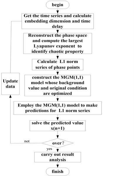
In the above paragraphs, the novel chaos prediction method based on MGM(1, 1) model, has been presented. The main idea of novel chaos prediction method is to transform predictions for the univariate time series into phase point predictions in reconstructed phase space with a MGM(1, 1) model. By studying the change law of Manhattan distance namely norm with MGM(1, 1) model, the proposed method is a novel method and distinctive. The Flow chart of forecasting algorithm is summarized as follows.
Fig. 1Flow chart of forecasting algorithm
5. Experimental results and analysis
5.1. The stabilized platform and the sample data
For showing the prediction capability and efficiency of the proposed MGM(1, 1) prediction model, take an actual stabilized platform system as an example to analyze. The stabilized platform is shown in Fig. 2. The stabilized platform consists of two level platforms witch include the bottom stabilized platform and the upper tracking platform. The bottom stabilization platform is mainly to reduce the disturbance of the external disturbance of the base, and provides a good level reference for target tracking. After ensuring the level of the base, the upper tracking platform can realize the effective tracking of the target. The stable platform system is drived by servo motor. Firstly, the adjusting shafts (pitch and yaw axis) of the bottom stabilized platform are contained by the main control computer with the control information (after calculation and processing of attitude adjustment information) of regulation to ensure stable layer approximation level. Secondly, the upper tracking platform according to the information of goal drives the servo motor for rotation of the azimuth and pitch regulation so as to achieve the goal of fast tracking. What’s more, the stable platform load is 30 kg, the bottom stabilized platform diameter is 450 mm, the frequency of stable platform is 1 Hz, the stable layer regulating shaft adjusting range is ±20°. The range of azimuth adjustment and pitch angle range of the upper tracking platform is 360°and ±5°respectively.
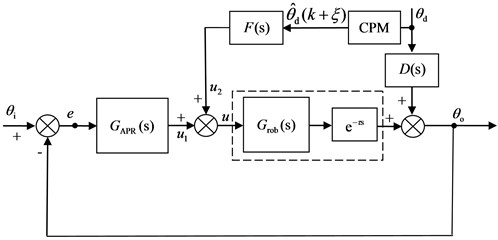
In Fig. 3, Signals , , denote the reference input, system output and tracking error of stabilized platform control system respectively. and is the regulator and object of position control respectively. is the link of time, is the carrier interference attitude, is the interference gallery transfer function and is the chaos time prediction module. The stabilized platform will be influenced by the carrier vibration interference attitude. Therefore, if the information of carrier vibration interference attitude can be obtained by prediction, the stabilized platform control system can suppress vibration interference in advance based on interference suppression. For this reason, the carrier vibration interference attitude prediction is very significant.
Fig. 2The stabilized platform
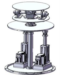
Fig. 3The compound control system structure
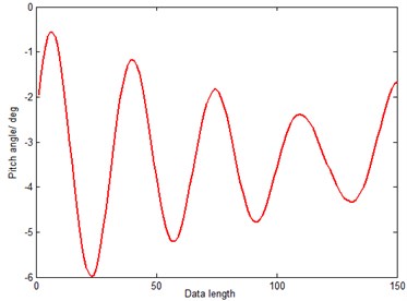
The sample data of carrier interference attitude are measured at a sampling frequency of 50 Hz with an Innalabs Attitude and Heading Reference System (AHRS) in a stabilized platform experiment. The data length is 1000. Take pitch attitude to analyze, the former 850 data are employed as training samples and latter 150 data are used as testing samples. The raw sample time series is shown in Fig. 4, the former 850 data and the latter 150 data are shown in Fig. 5 and Fig. 6.
Fig. 4Raw time series of pitch attitude
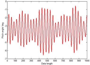
Fig. 5The former 850 points of sample data
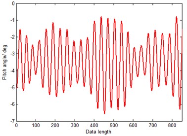
Fig. 6The latter 150 points of sample data
Before reconstructing the phase space, the pitch attitude series should be judged by the largest Lyapunov exponent method. Table 1 shows the largest Lyapunov exponent is greater than zero to prove that the pitch attitude series is chaotic and can be analyzed with chaotic methods.
Table 1The chaos property identification of raw time series
Length of the former data | The largest Lyapunov exponent | Time delay | Embedding dimension |
850 | 0.0037496 | 7 | 13 |
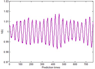
By reconstructing the phase space with time delay and embedding dimension , the L1 norm series of phase points can be obtained from Eq. (28) and the curve of L1 norm series is illustrated in Fig. 7. From Figs. 4 and 7, we can see that raw time series and L1 norm series are both oscillatory. Before predicting, class ratios should be examined. Since the raw time series of pitch attitude is not a nonnegative time sequence, it is preprocessed with upward translation in order to make the L1 norm series within the interval [33] as is shown in Fig. 6. The latest five points are employed to construct grey models, and the interval of class ratios would be . From Fig. 8 we can see that, the class ratios of roll attitude series after upward translation and L1 norm series all lie in the interval . In order to compare the performances of GM(1, 1) model, residual GM(1, 1) mode (RGM) [6] and the modified GM(1, 1) model (MGM) for oscillatory sequences, firstly of all, the three models are formed with raw time series respectively. Then five other chaotic prediction methods, Tang’s method (method 1), adding-weight one-rank local-region method (method 2), GM(1, 1) model applied in reconstructed phase space (method 3), residual GM(1, 1) model applied in reconstructed phase space(method 4), the combined forecasting model (method 5) [26] and the proposed MGM(1, 1) model applied in reconstructed phase space (method 6) proposed in the paper are used to predict the latter 150 sample points respectively.
Fig. 7L1 norm series
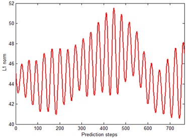
Fig. 8Class ratios of L1 norm series
5.2. Simulation results
In comparisons with the actual pitch data series curves, Figs. 9, 10 and 11 depict the predicted pitch attitude curves using GM(1, 1) model, residual GM(1, 1) model and MGM(1, 1) model respectively. And in order to compare the prediction method proposed in the paper with other mentioned methods, three criteria that contain the mean absolute percent error (MAPE), root mean square error (RMSE) and forecasting effective measure(FEM) are employed here [6].
Form Fig. 9 we can see that, big errors always exist at the inflexions by predicting with GM(1, 1) model. In Fig. 10, the large errors have been controlled when predicting with the residual GM(1, 1) model in a certain extent. On the contrary, when predicting with MGM in Fig. 11, errors can be reduced to a large certain extent at the inflexions due to optimizing background value and original condition. The prediction evaluation index is shown in Table 2, the overall performance of MGM is superior to GM(1, 1) model and residual GM(1, 1) model. Therefore we can conclude that, the MGM(1, 1) model would have a better performance for oscillatory sequences.
Fig. 9Prediction curve of GM(1, 1)
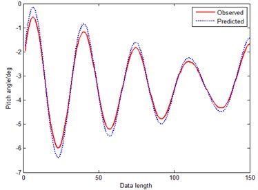
Fig. 10Prediction curve of RGM(1, 1)
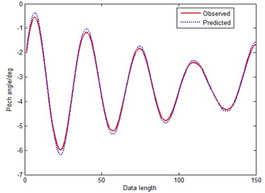
Fig. 11Prediction curve of MGM(1, 1)
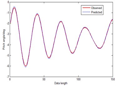
Table 2Evaluation results of prediction models
Prediction method | MAPE | RMSE | FEM |
GM(1, 1) | 0.02805 | 0.1905 | 0.81046 |
RGM(1, 1) | 0.02146 | 0.1685 | 0.85438 |
MGM(1, 1) | 0.01731 | 0.1264 | 0.91047 |
Method 1 | 0.57394 | 3.8276 | 0.20572 |
Method 2 | 0.29146 | 0.6023 | 0.57351 |
Method 3 | 0.020832 | 0.1634 | 0.91852 |
Method 4 | 0.017854 | 0.1013 | 0.95878 |
Method 5 | 0.018375 | 0.1356 | 0.94862 |
Method 6 | 0.014764 | 0.0938 | 0.97986 |
Figs. 12-17 are prediction curves of each model, and Table 2 lists the evaluation results.
Figs. 12-17 depict predictions made from reconstructed phase space. From above figures, we can see that method 1 has the worst prediction performance in Fig. 12, and the evaluation results indicate that it is not fit for the attitude prediction of stabilized platform. Fig. 13 indicates that the performance of adding-weight one-rank local-region method is quite unstable because it is a simple prediction method. Compare Fig. 12 with Fig. 13, we can find that method 2 is better than method 1. AOLM finds a set of neighbor points in reconstructed phase space, and constructs a first-order linear model. Then adopt least square method to estimate the model coefficients with these neighbor points, and system prediction model would be obtained in this way. The poor capability of AOLM may be due to its first-order linear model, hence choosing a proper model in reconstructed phase space is also very important. When comparing method 6 with method 1 and method 2, we can see that there is no bad prediction inflexion in Fig. 16 which exists in Fig. 12 and Fig. 13. And Table 2 shows that, MAPE and RMSE of method 5 are almost decuple better than the method 1 and method 2, and FEM is high to 0.97986.
Fig. 12Prediction curve of Tang’s method (method 1)
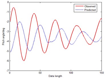
Fig. 13Prediction curve of AOLM (method 2)
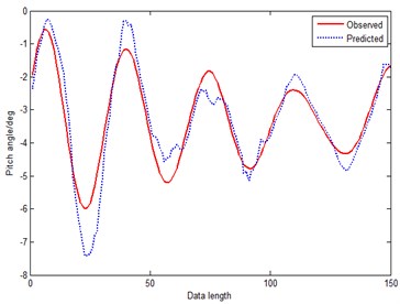
Fig. 14Prediction curve of GM-RPS (method 3)
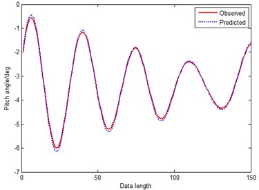
Fig. 15Prediction curve of RGM-RPS (method 4)
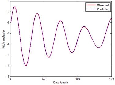
Fig. 16Prediction curve of CFM (method 5)
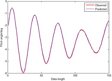
Fig. 17Prediction curve of MGM-RPS (method 6)
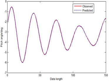
By comparing Figs. 14, 15 and 16 with Figs. 9, 10 and 11, we can find, that predictions made in reconstructed phase space substantially reduce the errors of GM(1, 1), residual GM(1, 1) model and MGM predictors. GM-RPS is better than GM(1, 1) obviously, and evaluation results show that its performance is almost equivalent to MGM. What’s more, RGM-RPS is superior to RGM and GM distinctly. By comparing Fig. 14, with Fig. 15, the RGM-RPS is better than GM-RPS, because the RGM-RPS has compensated the predicted value by counting residual series to improve the prediction precision. By comparing Figs. 14, 15 with Fig. 16 respectively, among the three methods, MGM-RPS is the best with no doubt. MGM-RPS has not only compensated the predicted value, but also optimized background value and optimized original condition. Furthermore, in Table 2, we can see that MAPE and RMSE of method 5 are almost decuple better than the method 3 and method 4 too. MAPE and RMSE of method 3 are 0.020832 and 0.1634, and MAPE and RMSE of method 4 are 0.017854 and 0.1013 respectively. However, the MAPE and RMSE of method 5 are only 0.014764 and 0.0938.
When comparing Fig. 16 with Fig. 17, the prediction performances shown in Table 2 exhibit that, the MAPE and RMSE of method 5 is bigger than the method 6. And the computational cost of method 5 is high. The overall performance of MGM-RPS is distinctly superior to combined forecasting model. Consequently we can reach a conclusion with no doubt: the newly proposed chaos prediction method with MGM(1, 1) model applied in reconstructed phase space could effectively extract the chaotic time series features.
6. Conclusions
A novel chaos time series prediction model is presented in this paper. With combining chaotic theory – GM(1, 1) model and phase space reconstruction technique, one-dimension time series of pitch attitude is developed to multi-dimension phase space, which contains the reconstructed chaotic attractor preserving both geometrical and dynamical properties of the original chaotic attractor. And then MGM(1, 1) model rather than GM(1, 1) model is employed to study evolution laws of the L1 norm series in reconstructed phase space, a modified GM(1, 1) (MGM(1, 1)) model is proposed mainly by optimizing background value and optimizing original condition. Empirical results indicate that, the MGM(1, 1) model is more suitable for oscillatory sequence than GM(1, 1) model, and the chaos prediction method with MGM(1, 1) model applied in reconstructed phase space is effective and practical for the attitude prediction. Especially when higher prediction accuracy is needed, the approach of MGM-RPS brings a new selection for chaos time series prediction task. The empirical results of stabilized platform are encouraging and indicate that the newly proposed method is excellent in prediction of chaos time series of chaos systems.
7. Future work
The next step of our research efforts will be the research of optimizing parameters in prediction of chaos time series. Such as, embedding dimension in the phase space reconstruction can be obtained by using non-embedding techniques [34]. As we know, non-uniform embedding (when time delays are not all equal) are surpassing uniform embeddings. On the base of non-embedding techniques and through the use of non-uniform embedding method to select the embedding dimension in the phase space reconstruction, we compare the non-uniform embedding method with uniform embedding method combined with MGM prediction algorithm in article, and try on the stable platform system. What’s more, the joint optimization of parameters in prediction method will be considerable and the joint optimization MGM algorithm will be the important direction for our future research.
References
-
Khashei M., Bijari M. A new class of hybrid models for time series forecasting. Expert Systems with Applications, Vol. 39, 2012, p. 4344-4357.
-
Gao C., Qian J. Evidence of chaotic behavior in noise from industrial process. Transactions on Signal Processing, Vol. 36, Issue 6, 2007, p. 2877-2884.
-
Wu H., Jiang C., Tai N., Hou Z. The application of grey neural network model to city electricity demand forecasting. The Journal of Grey System, Vol. 4, 2004, p. 357-365.
-
Yang W., Liu S., Wang Y. The grey prediction of change trend of Chinese financial industry’s credit size. The Journal of Grey System, Vol. 1, 2006, p. 67-74.
-
Chen Z., Li L., Xiao X. GM(1, 1) model and its application to controlling the inverted camber of widening concrete bridge. The Journal of Grey System, Vol. 4, 2006, p. 365-374.
-
Lu J., Wang C. M., Zhang A. J., Xie X. M. Residual GM(1, 1) model-based prediction method for chaotic time series. The Journal of Grey System, Vol. 4, 2012, p. 379-388.
-
Truong D. Q., Ahn K. K. An accurate signal estimator using a novel smart adaptive grey model SAGM(1, 1). Expert Systems with Applications, Vol. 39, 2012, p. 7611-7620.
-
Lu J., Xie W., Zhang A., Wang C. Chaos-based modified GM(1, 1) power model in time series prediction. The Journal of Grey System, Vol. 26, Issue 4, 2014, p. 32-43.
-
Lu J., Xie W., Zhou H., Zhang A. Vibration suppression using fractional-order disturbance observer based adaptive grey predictive controller. Journal of Vibroengineering, Vol. 16, Issue 5, 2014, p. 2204-2215.
-
Kayacan E., Kaynak O. Single-step ahead prediction based on the principle of concatenation using grey predictors. Expert Systems with Applications, Vol. 38, 2011, p. 9499-9505.
-
Zhan Y., Ding Y., Cheng H. Improving GM(1, 1) model in support vector machines. The Journal of Grey System, Vol. 1, 2005, p. 45-50.
-
Zeng B., Liu S. F. Prediction model of stochastic oscillation sequence based on amplitude compression. Systems Engineering – Theory and Practice, Vol. 32, Issue 11, 2012, p. 2493-2497.
-
Wang Z., Hipel K., Wang Q. An optimized NGBM(1, 1) model for forecasting the qualified discharge rate of industrial wastewater in China. Applied Mathematical Modeling, Vol. 35, 2011, p. 5524-5532.
-
Wang Z., Dang Y., Liu S. An optimal GM(1, 1) based on the discrete function with exponential law. Systems Engineering – Theory and Practice, Vol. 28, Issue 2, 2008, p. 61-67.
-
Zhang B., Xi G. GM(1, 1) model optimization based on the background value and boundary value correction. Systems Engineering – Theory and Practice, Vol. 33, Issue 3, 2013, p. 682-688.
-
Yao T., Liu S., Dang Y. Discrete grey prediction model based on optimized initial value. Systems Engineering – Theory and Practice, Vol. 31, Issue 10, 2009, p. 239-2398.
-
Wang F. Unequal interval grey forecast models based on the modificatory initial-value. Journal of Chongqing Normal University, Vol. 23, Issue 3, 2006, p. 42-44.
-
Zhang Y., Wei Y., Zhou P. Improving grey derivative GM(1, 1). The Journal of Grey System, Vol. 18, Issue 4, 2006, p. 375-380.
-
Li B., Wei Y. Optimizes grey derivative of GM(1, 1). Systems Engineering – Theory and Practice, Vol. 29, Issue 2, 2009, p. 100-105.
-
Cui J., Dang Y., Cui Z. Analysis on modeling accuracy of GM(1, 1) based on new weakening operators. Systems Engineering – Theory and Practice, Vol. 29, Issue 7, 2009, p. 132-138.
-
Wu Z., Liu S., Cui L. Study on new weakening buffer operators. Control and Decision, Vol. 24, Issue 12, 2009, p. 1805-1809.
-
Lü J., Lu J., Chen S. Chaotic Time Series Analysis and Its Applications. Wu Han, Wu Han University Publication, 2002.
-
Maguire L., Roche B., McGinnity T. Predicting a chaotic time series using a fuzzy neural network. Information Sciences, Vol. 112, Issue 1, 1998, p. 125-136.
-
Tang Q. Grey-chaos method of experiment data processing and its application. Machine Tool and Hydraulics, Vol. 3, Issue 1, 2003, p. 262-264.
-
Li X., Liu Z. Research on grey prediction of deformation laws in backfill based on phase space reconstruction. Journal of Safety and Environment, Vol. 4, Issue 6, 2004, p. 54-57.
-
Lu J., Wang C., Zhang A. Hierarchical combined forecasting based on L1 norm of reconstructed phase points. Journal of Nanjing University of Science and Technology, Vol. 37, Issue 2, 2013, p. 286-290.
-
Zhang B., Xi G. GM(1, 1) model optimization based on the background value and boundary value correction. Systems Engineering – Theory and Practice, Vol. 33, Issue 3, 2013, p. 682-688.
-
Kim H., Eykholt R., Salas J. Nonlinear dynamics, delay times, and embedding windows. Physica D, Vol. 127, 1999, p. 48-60.
-
Brock W., Hsieh D., LeBaron B. Nonlinear Dynamics, Chaos, and Instability: Statistical Theory and Economic Evidence. MIT Press, Cambridge, MA, 1991.
-
Lv J., Lu J., Chen S. Chaotic Time Series Analysis and Its Application. Wu Han University Press, Wu Han, 2002, p. 102-104.
-
An X., Jiang D., Liu C., Zhao M. Wind farm power prediction based on wavelet decomposition and chaotic time series. Expert Systems with Applications, Vol. 38, 2011, p. 11280-11285.
-
Chen H., Liu C. Properties of weighted geometric means combination forecasting model based on L1 norm. Journal of Southeast University (Natural Science Edition), Vol. 34, Issue 4, 2013, p. 535-540.
-
Deng J. Grey System Fundamental Method. HUST Press, Wuhan, 1982.
-
Ragulskis M., Lukoševičiūtė K. Non-uniform attractor embedding for time series forecasting by fuzzy inference systems. Neurocomputing, Vol. 72, Issues 10-12, 2009, p. 2618-2626.
About this article
The research is supported by the National High Technology Research and Development Program of China (863 Program) (Grant No. 2012AA061101), the Open Project Program of Key Laboratory of Intelligent Perception and systems for High-Dimensional Information (Grant No. 30920130122005), and Research Fund for Doctoral Program of Higher Education of China (No. 20133219110027).
The authors wish to express their deep appreciation to Mr. Lu jianshan of Vehicle Engineering Research Institute of Zhejiang University of Technology and Mr. Yan shun of Nanjing University of Science and Technology, for their contribution in the test experiment efforts.
