Bearing fault diagnosis method based on Hilbert envelope spectrum and deep belief network

Wang, Xingqing; Li, Yanfeng; Rui, Ting; Zhu, Huijie; Fei, Jianchao

Journal of Vibroengineering

Browse Journal

Submit article

Published: 15 May 2015

Check for updates

Bearing fault diagnosis method based on Hilbert envelope spectrum and deep belief network

Xingqing Wang¹

Yanfeng Li²

Ting Rui³

Huijie Zhu⁴

Jianchao Fei⁵

^{1, 2, 3, 4, 5}College of Field Engineering, People’s Liberation Army University of Science and Technology, Nanjing, China

Corresponding Author:

Yanfeng Li

Cite the article Download PDF

Downloads 1603

WoS Core Citations 30

Abstract

When fault occurs in bearing, the frequency spectrum of vibration signal would change and it contains a considerable amount of fault information which can reflect the actual work condition and the fault type of bearing. Recently, the statistical features of the frequency spectrum have been widely used in bearing fault diagnosis. However, there are lots of statistical features with different sensitivity to fault identification. Selecting the most sensible statistical features for improving classification accuracy is often determined with experience, which will make great subjective influence on the fault diagnosis results. Deep belief network (DBN) is a deep neural network which can automatically find a latent hierarchical feature representation from the high dimension input data. In this study, a bearing fault diagnosis method based on Hilbert envelope spectrum and DBN is proposed. Firstly, the vibration signals under different test conditions are resampled. Secondly, the whole Hilbert envelope spectrum of the resampled signal is used directly as eigenvector to characterize the fault type of bearing. Finally, a DBN classifier model is established to recognize the fault type of bearing. DBN classifier model can be used as both an automatic feature extractor and a classifier for bearing fault diagnosis. Therefore, the process of fault diagnosis can be greatly simplified. The results of two different experiments demonstrate that the proposed method outperforms the competing methods and it can obtain a more excellent diagnostic performance.

1. Introduction

As an important component, bearing is widely used in rotating machinery. The condition of bearing influences the reliability of rotating machinery greatly. Statistics has shown that the majority of problems in rotating machinery arise from the faulty bearings [1, 2]. When fault occurs in bearing, it may lead to fatal breakdown and serious damage. Therefore, it is of great importance to accurately detect and diagnose the fault type of bearing.

Generally speaking, there are two main kinds of bearing fault diagnosis methods: signal processing-based fault diagnosis method and artificial intelligence-based fault diagnosis method. Signal processing-based fault diagnosis method is an effective and powerful tool in bearing fault diagnosis, but it requires considerable expertise to judge the fault type of bearing. Recently, artificial intelligence-based fault diagnosis method has received increasing attention because it doesn’t need so much expertise and could achieve a high degree of accuracy.

Artificial intelligence-based fault diagnosis method usually contains two steps: feature extraction and fault pattern recognition. Many feature extraction methods have been proposed, such as sparse representation [3], wavelet transform [4], wavelet leaders multi-fractal [5], empirical mode decomposition (EMD) [6, 7], morphological analysis [8], singular value decomposition (SVD) [9] and so on. When fault occurs in bearing, the frequency spectrum of vibration signal would change and it contains a considerable amount of fault information which can reflect the actual work condition and the fault type of bearing. Recently, the statistical features of the frequency spectrum have received increasing attention. Zhu et al. [10] used the statistical features of the raw vibration signal, the frequency-domain and the Hilbert envelope spectrum for bearing performance assessment. Liu et al. [11] applied EMD to vibration signals and extracted some statistical features from several intrinsic mode functions (IMFs) both in time and frequency domain for bearing fault diagnosis. There are lots of statistical features with different sensitivity to fault identification. Due to excessive irrelevant statistical features extracted from the frequency spectrum, PCA [12], decision tree [13], distance evaluation technique (DET) [14-15] and many other feature selection methods are used to get the most sensitive features for further improving the fault diagnosis accuracy. Selecting the most sensible statistical features of frequency spectrum is often determined with experience, which will make great subjective influence on the fault diagnosis results. To tackle this problem, the Hilbert envelope spectrum of the vibration signal is used directly to construct the feature vector of bearing in this study.

Pattern recognition is another crucial step of Artificial intelligence-based fault diagnosis method. Artificial neural networks (ANN) [16] and support vector machine (SVM) [17] are the most widely used classifiers. But these traditional classifiers are shallow architectures which have some drawbacks including local optimal solution, slow convergence and time-consuming. The dimension of the feature vector based on Hilbert envelope spectrum is usually very high, the shallow architectures are not suitable to deal with the high dimension input data. Deep belief network (DBN) is a deep neural network and it simulates the human brain to recognize objects through different layers’ features. In recent years, DBN have been successfully used in digit recognition [18], acoustic representation [19], time series forecasting [20], soft sensor modeling [21], compressor valves fault diagnosis [22]. However, the implementation of DBN in bearing fault diagnosis is still uncommon.

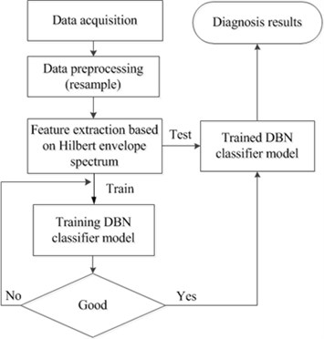
In this study, a new bearing fault diagnosis method based on Hilbert envelope spectrum and DBN is proposed. The schematic diagram of bearing fault diagnosis is shown in Fig. 1. The vibration signal under different test condition is firstly resampled at the frequency $m$ times the rotating frequency of bearing. Then, the Hilbert envelope spectrum of the resampled signal is used to construct the feature vector. Finally, a DBN classifier model is established to recognize the bearing fault types.

Fig. 1The flowchart of bearing fault diagnosis

The rest of this paper is organized as follows: Section 2 gives a brief description of the feature extraction method based on Hilbert envelope spectrum. In Section 3, the basic components of DBN including restricted Boltzmann machine (RBM) and Gaussian restricted Boltzmann machine (Gaussian RBM) are introduced, and a DBN classifier model is established for bearing fault diagnosis. In Section 4, the effectiveness of the proposed method is demonstrated with two different experiments. Finally, conclusions are drawn in Section 5.

2. Feature extraction method based on Hilbert envelope spectrum

When fault occurs in bearing, the vibration signal would change. Additionally, the Hilbert envelope spectrum and its distribution may have some variations. For the vibration signal $x$ , its Hilbert transform is:

1

H [x] = \frac{1}{π} \int_{- \infty}^{+ \infty} \frac{x}{t - τ} d τ .

The Hilbert envelope spectrum can be given as:

2

h (f) = \frac{1}{π} \int_{- \infty}^{+ \infty} \sqrt{x^{2} + H^{2} [x]} e^{- j 2 π f t} d t .

The Hilbert envelope spectrum of vibration signal contains a considerable amount of fault information which can reflect the actual work condition and the fault pattern of bearing. Many researches have demonstrated that the statistical features of the Hilbert envelope spectrum can be used for bearing assessment [10]. There are lots of statistical features with different sensitivity to fault identification, selecting the most sensitive features needs considerable expertise. To tackle this problem, the Hilbert envelope spectrum of the vibration signal is used directly to construct the feature vector. Because the feature vector is influenced greatly by the speed, to make the feature vector more robust, here we propose a new features extraction method and the main steps can be described as follows:

Step 1, resample the vibration signal $x$ with the sample frequency $m f_{R}$ Hz. Here $f_{R}$ is the rotating frequency of bearing and $m$ is a real number. By resampling, we can get $m$ sample points every revolution of bearing. Therefore, the influence of different speeds can be reduced. In the resampling process, an anti-aliasing (low-pass) FIR filter is applied to compensate for the signal delay.

Step 2, calculate the Hilbert envelope spectrum $h (f)$ of the resampled signal $x^{'}$ . The length of $x^{'}$ is chosen as $N$ in this study.

Step 3, construct the feature vector $T$ by the Hilbert envelope spectrum $h (f)$ directly:

3

T = [h (f_{1}), h (f_{2}), \dots, h (f_{K})],

where $h (f_{k})$ is the Hilbert envelope spectrum for $k =$ 1,…, $K$ . $K$ is the number of the Hilbert envelope spectrum lines and it is usually equal to $N / 2$ .

Step 4, repeat Step 1-3 and get the feature vectors of all vibration signals.

3. DBN classifier model

The dimension of the feature vector based on Hilbert envelope spectrum is usually very high and there is a ‘curse of dimensionality’ problem when using the traditional classifiers. To deal with the high dimension input data, a DBN classifier model is established in Section 3. The DBN classifier model can be used as both an automatic feature extractor and a classifier for bearing fault diagnosis. Therefore, the process of bearing fault diagnosis can be greatly simplified. In Section 3.1, the basic components of DBN including RBM (restricted Boltzmann machines) and Gaussian RBM are introduced. In Section 3.2, a DBN classifier model is established and its training process is described briefly.

3.1. RBM and Gaussian RBM

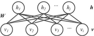
As the basic component of DBN, RBM has attracted increasing attention for its ability to provide a closed-form representation of the distribution underlying the high dimension data. RBM can be viewed as non-linear feature detectors [23]. As shown in Fig. 2, RBM is a bipartite undirected graphical model that consists of a visible layer $v$ and a hidden layer $h$ . For the two layers in RBM, all visible units are connected to all hidden units, and there are no connections between any two units within the same layer. In RBM, all the units in the visible layer and hidden layer are binary stochastic units. The architecture of Gaussian RBM is the same as that of RBM, but its visible units are linear units with independent Gaussian noise. Compared with RBM, Gaussian RBM is much more convenient for modeling real-valued data [24].

Fig. 2The architecture of RBM (Gaussian RBM)

RBM is an energy-based stochastic neural network and the energy function of the visible layer $v$ and the hidden layer $h$ is defined as:

4

E (v, h) = - \sum_{i} a_{i} v_{i} - \sum_{j} b_{j} h_{j} - \sum_{i, j} v_{i} h_{j} w_{i j},

where $v_{i}$ and $h_{j}$ are the binary state of visible unit $i$ and hidden unit $j$ , $w_{i j}$ is the weight between them, $a_{i}$ and $b_{j}$ are the biases.

The joint distribution over the visible layer $v$ and the hidden layer $h$ is based on energy function and it can be formulated as:

5

p (v, h) = \frac{1}{Z} e x p (- E (v, h)),

where $Z = \sum_{v, h} e x p (- E (v, h))$ is the normalizing factor.

Therefore, the probability that RBM assigns to the visible layer $v$ is:

6

p (v) = \frac{1}{Z} \sum_{h} e x p (- E (v, h)) .

Because there are no connections in the same layer of RBM, the conditional probability $p (h | v)$ and $p (v | h)$ can be given by:

7

p (h_{j} = 1 | v) = σ (b_{j} + \sum_{i} v_{i} w_{i j}),

8

p (v_{i} = 1 | h) = σ (a_{i} + \sum_{j} h_{j} w_{i j}),

where $σ (x) = 1 / (1 + e x p (- x))$ is a sigmoid function.

The training process of RBM is based on stochastic gradient descent and it can be realized by maximizing $p (v)$ which is the probability of the model simply on the training data. The gradient of the negative log probability of the visible layer $v$ with respect to the model parameters $θ = \{w_{i j}, a_{i}, b_{j}\}$ can be obtained from:

9

\frac{\partial p (v)}{\partial w_{i j}} = {〈v_{i} h_{j}〉}_{d a t a} - {〈v_{i} h_{j}〉}_{m o d e l},

10

\frac{\partial p (v)}{\partial a_{i}} = {〈v_{i}〉}_{d a t a} - {〈v_{i}〉}_{m o d e l},

11

\frac{\partial p (v)}{\partial b_{j}} = {〈h_{j}〉}_{d a t a} - {〈h_{j}〉}_{m o d e l},

where ${〈∙〉}_{d a t a}$ denotes the expectation with respect to the training data’s distribution, ${〈∙〉}_{m o d e l}$ denotes the expectation with respect to the distribution defined by the model.

According to Eq. (9)-(11), the update rule of the parameters is given as:

12

∆ w_{i j} = ε {(〈v_{i} h_{j}〉}_{d a t a} - {〈v_{i} h_{j}〉}_{m o d e l}),

13

∆ a_{i} = ε ({〈v_{i}〉}_{d a t a} - {〈v_{i}〉}_{m o d e l}),

14

∆ b_{j} = ε ({〈h_{j}〉}_{d a t a} - {〈h_{j}〉}_{m o d e l}),

where $ε$ is the learning rate.

It is very easy to get the unbiased sample of ${〈∙〉}_{d a t a}$ . However, the unbiased sample of ${〈∙〉}_{m o d e l}$ is intractable to compute. In many applications, a fast learning procedure based on contrastive divergence (CD) is used [24]. It starts by setting the states of the visible units to a training data. Then the binary states of the hidden units are all computed in parallel using Eq. (7). Once the binary states have been chosen for the hidden units, a “reconstruction” is produced by setting each $v_{i}$ to 1 with a probability given by Eq. (8). The change of the parameters is given by:

15

∆ w_{i j} = ε {(〈v_{i} h_{j}〉}_{d a t a} - {〈v_{i} h_{j}〉}_{r e c o n}),

16

∆ a_{i} = ε ({〈v_{i}〉}_{d a t a} - {〈v_{i}〉}_{r e c o n}),

17

∆ b_{j} = ε ({〈h_{j}〉}_{d a t a} - {〈h_{j}〉}_{r e c o n}) .

It is possible to update the parameters after estimating the gradient on a single training set. But it is often more efficient to divide the training set into small “mini-batches” of several cases. To avoid having to change the learning rate when the size of a mini-batch is changed, it is helpful to divide the total gradient computed on a mini-batch by the size of the mini-batch [24].

Gaussian RBM’s visible units are linear units with independent Gaussian noise, so its energy function is different from that of RBM:

18

E (v, h) = - \sum_{i} \frac{{(v_{i} - a_{i})}^{2}}{2 {σ_{i}}^{2}} - \sum_{j} b_{j} h_{j} - \sum_{i, j} \frac{v_{i}}{σ_{i}} h_{j} w_{i j},

where $σ_{i}$ is standard deviation of the visible unit $v_{i}$ .

The probability that Gaussian RBM assigns to the visible layer $v$ is given as follows:

19

p (v, h) = \frac{1}{Z} \exp (- E (v, h)),

where $Z = \int \sum_{h} e x p (- E (v, h))$ .

For Gaussian RBM, the conditional probability can be expressed as:

20

p (h_{j} = 1 | v) = σ (b_{j} + \sum_{i} v_{i} w_{i j}),

21

p (v_{i} = x | h) = \frac{1}{σ_{i} \sqrt{2 π}} e x p (\frac{{(x - a_{i} - σ_{i} \sum_{j} h_{j} w_{i j})}^{2}}{2 {σ_{i}}^{2}}),

where $x$ is a real number.

The training process of Gaussian RBM is similar to RBM and it is also based on stochastic gradient descent. In practical use, the input data of Gaussian RBM is commonly normalized to have zero mean and unit variance by a linear transformation [21]. This makes more simplicity of the model implementation.

3.2. DBN classifier model and its training process

As shown in Fig. 3, DBN is formed by a series of RBMs which are stacked layer by layer. DBN with $L$ hidden layers can be trained in an unsupervised way with the greedy layer-wise procedure, in which each added layer is trained as an RBM by contrastive divergence algorithm. The training process of DBN can be described as follows:

Step 1, initialize all the parameters of DBN stochastically.

Step 2, use the input data to train the bottom RBM by contrastive divergence algorithm.

Step 3, use the output of the low-level RBM as the input data to train the high-level RBM.

Step 4, repeat Step 3 until all the RBMs are trained.

The special architecture and training process make DBN have the ability to retrieve features directly from the input data. The extracted features are more suitable for classification than the input data. In this study, Gaussian RBM is used as the bottom RBM for its better ability to model the real-valued input data than RBM.

After unsupervised training process, the parameters $\{W_{l}, a_{l}, b_{l}\}$ $(l =$ 1,…, $L)$ of the pre-trained DBN can be obtained. By adding an extra layer $o$ of variables that represent the labels of the training data, we can get a DBN classifier model. The training process of the DBN classifier model is also shown in Fig. 3. The weights of the DBN classifier model are set the same as $\{W_{l}, b_{l}\}$ $(l =$ 1,…, $L)$ except the top layer. The weights ${W_{L + 1}, b_{L + 1}}$ between the hidden layer $h_{L}$ and the top layer $o$ are initialized stochastically. Then, the training data with labels are used to train the DBN classifier model by back-propagation algorithm in a supervised way.

Fig. 3The DBN classifier model and its training process

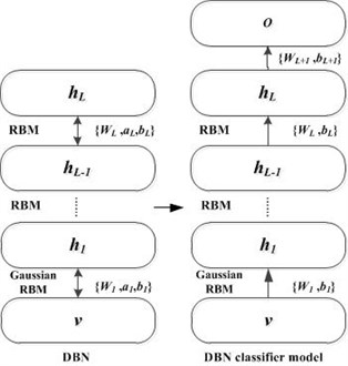
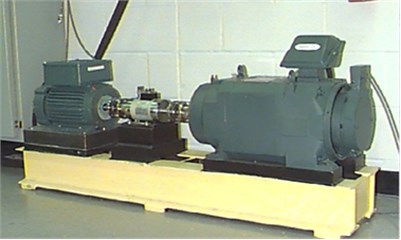
Fig. 4The bearing test stand

4. Experimental verification of the proposed bearing fault diagnosis method

In order to verify the proposed fault diagnosis method, the bearing vibration data collected from two different experiments are analyzed in this section. In the first experiment, the bearing vibration data is obtained from the Case Western Reserve University Bearing Data Center [25]. The test bearings are installed in an induction motor. Each bearing with only a single fault is tested under four different loads. In the second experiment, the test bearings are installed in a hydraulic piston pumps. The test bearings have different fault types including both signal faults and multiple faults. All the bearings are tested under two different loads. Details about the two experiments will be described in the following section.

4.1. Experiment 1: Bearing fault diagnosis for induction motor

4.1.1. Experiment introduction

The bearing vibration data obtained from the Case Western Reserve University Bearing Data Center is collected from the bearing test stand as shown in Fig. 4. The test stand consists of a 2 hp (1 hp $=$ 0.735 kW) induction motor, a torque transducer, accelerometers, a dynamometer and so on. The type of the bearing used in the experiment is 6205 SKF. Single faults with fault diameters of 0.18 mm, 0.36 mm, 0.53 mm respectively are introduced to the driving end bearings using the electric discharge machining method. The bearings with different fault diameters are tested under 0, 1, 2 and 3 hp loads. The speeds of the motor under different loads are 1797, 1772, 1750, 1730 rpm, respectively. An accelerometer is mounted on the motor housing at the drive end of the motor to acquire the vibration signals from the test bearing. Vibration signals are collected by a data recorder with the sample frequency of 12 kHz.

4.1.2. Feature extraction

The normal bearing and nine other fault bearings with the fault diameter of 0.18 mm, 0.36 mm, 0.53 mm are used in this study. All the bearings are tested under four different loads. Each vibration signal $x$ is a time-series with 2400-point window block, and there is no overlap between any two vibration signals.

In the experiment, the speeds of bearing would change under different loads. The rotating frequencies $f_{R 1}$ , $f_{R 2}$ , $f_{R 3}$ , $f_{R 4}$ are 29.95, 29.53, 29.17, 28.83 Hz, respectively. According to the feature extraction method described in Section 2, the vibration signal $x$ is resampled at the frequency which is $m$ times the rotating frequency $f_{R i}$ ( $i =$ 1, 2, 3, 4) Hz. Then, the first $N$ points of the resampled signal are used to calculate the Hilbert envelope spectrum. After that, the Hilbert envelope spectrum is used directly to construct the feature vector. In this experiment, the parameters $m$ , $N$ are chosen as 400 and 2000, respectively. Therefore, the dimension of the feature vector is 1000. Take the normal bearing and three bearings with the fault diameter of 0.18 mm for example, the feature vectors under four different loads are shown in Fig. 5. From these figures, it is easy to see that, the feature vectors of the same fault type are close to each other, while the feature vectors of different fault types can be clearly distinguished. Fig. 5 also demonstrates that the feature vectors are robust and insensible to different speeds and loads.

4.1.3. Classification performance of the proposed method

Select 40 samples (feature vectors) for ten different bearings under four different loads and we can get a bearing data set including 800 samples. 400 samples are randomly selected for training the DBN classifier model and the rest 400 samples are used for testing. The detailed description of the bearing data set in Experiment 1 is shown in Table 1.

A DBN classifier model with two hidden layers is used for bearing fault diagnosis. For the DBN classifier model, the two hidden layers have the same number of hidden units. The size of the mini-batch is set to 10, which is equal to the number of bearing categories. The learning rate $ε$ is fixed at 0.0001 as suggested by Hinton. The max epoch for the RBM (or Gaussian RBM) training process and the back-propagation learning process are chosen as 50 and 100, respectively. To account for the stochastic nature of the DBN classifier model, the classification process is repeated for 10 times and the results are averaged.

Table 2 lists the classification results acquired by the DBN classifier models with different number of hidden units. The number of hidden units ranges from 10 to 100. From the results in Table 2, it can be seen that all the training accuracies are 100 % except for the DBN classifier model with 10 hidden units (95.13 %). The testing accuracy of the DBN classifier model with 10 hidden units is 92.98 %. For the DBN classifier models which have no less than 20 hidden units, the testing accuracies range from 98.7 % to 99.55 %. The DBN classifier model with 10 hidden units doesn’t perform as well as the other DBN classifier models. The main reason is that the DBN classifier model has too less hidden units and it can’t effectively learn the high complexity non-linear relationships between the input data (feature vector) and the bearing fault types. The results in Table 2 demonstrate that the proposed method is robust and can achieve a high degree of classification accuracy for bearing fault diagnosis.

Fig. 5The feature vectors of bearings with single faults (fault diameter: 0.18 mm) in Experiment 1

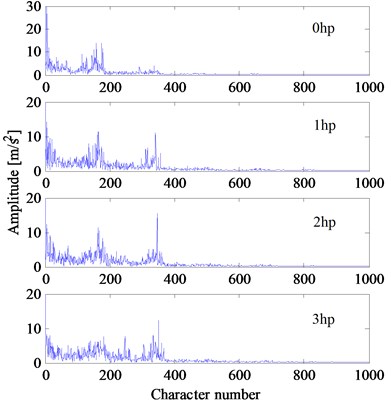
a) Normal

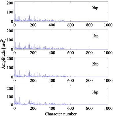
b) Inner race fault

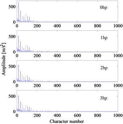
c) Outer race fault

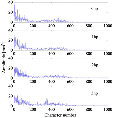
d) Ball fault

In this study, to demonstrate the superiority of the proposed method, three other traditional classifiers including K-nearest neighbors (KNN), support vector machine (SVM), extreme learning machine (ELM) are used for comparison experiment. For SVM, the kernel function is selected as Gaussian function. For ELM, the number of the hidden units is set to 1000. For KNN, the number of neighbors is set to 10 and the Euclidean distance is used. Fig. 6 shows the results of these classifiers. From the results in Fig. 6, it can be realized that the proposed method outperforms the other three traditional methods.

Table 1The description of the bearing data set in Experiment 1

Fault type	Fault diameter (mm)	Training samples	Testing samples	Classification label
Normal	0	40	40	1
Inner race	0.18	40	40	2
Outer race	0.18	40	40	3
Ball	0.18	40	40	4
Inner race	0.36	40	40	5
Outer race	0.36	40	40	6
Ball	0.36	40	40	7
Inner race	0.53	40	40	8
Outer race	0.53	40	40	9
Ball	0.53	40	40	10

Table 2The classification results of the DBN classifier model in Experiment 1

Number of hidden units	Training accuracy (%)	Testing accuracy (%)
10	95.13	92.98
20	100	98.7
30	100	99.2
40	100	99.28
50	100	99.53
60	100	99.33
70	100	99.48
80	100	99.38
90	100	99.5
100	100	99.55

Fig. 6The classification results obtained by different classifier models in Experiment 1

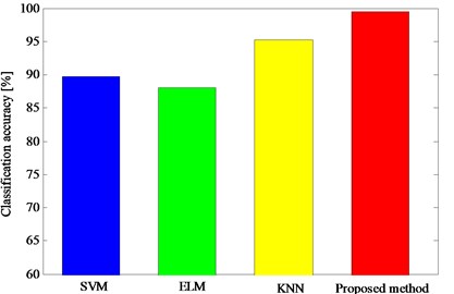
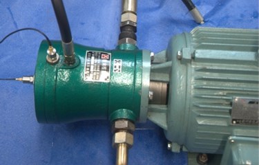
Fig. 7The hydraulic piston pump experiment system

4.1.4. Performance comparison of the proposed method and other published ones

The bearing vibration data obtained from the Case Western Reserve University Bearing Data Center has been wildly used to verify the performance of different bearing fault diagnosis algorithms [5, 26, 27]. Many researchers have proposed various feature extraction methods and classification algorithms. Hu et al. [26] combined the improved wavelet package energy features and SVMs ensemble (IWPE-SVME) for bearing fault diagnosis, although both feature selection technology and SVMs ensemble are used in [26], the classification accuracy of IWPE-SVME ranges from 97 % to 99 %, and it is inferior to that of the proposed fault diagnosis method (HES-DBN). In reference [5], the multi-fractal feature and wavelet package energy feature based SVMs (MF-SVMs) are proposed for bearing fault diagnosis and the classification accuracy for ten different bearing fault types under 1hp load is only 88.9 %. In reference [27], the classification accuracy of the frequency-domain feature based ANFIS (F-ANFIS) for ten different bearing fault types is only about 87.8 %. Both the results of MF-SVMs and F-ANFIS are inferior to that of the proposed H-DBN method. Table 3 gives the performance comparison of these aforementioned methods. For the proposed method in this paper, the fault diagnosis process is simple and robust. Besides, it can obtain a more excellent diagnostic performance.

Table 3The performance comparison of different bearing fault diagnosis methods

Reference	Method	Number of bearing fault types	Number of loads	Classification accuracy (%)
Hu et al.[26]	IWPE-SVME	7	4	97-99
Du et al. [5]	MF-SVMs	10	1	88.9
Lei et al. [27]	F-ANFIS	10	4	87.7
This paper	HES-DBN	10	4	99.55

4.2. Experiment 2: Bearing fault diagnosis for hydraulic piston pump

4.2.1. Experiment introduction

As an important component of the hydraulic piston pump, bearing supports the cylinder block and controls its movement in axial and radial directions. Due to harsh working environment and heavy working loads, single faults and multiple faults often occur in bearing, resulting in abnormal vibration in radial direction [28]. Due to the complicated structure-borne vibration and fluid-borne vibration of hydraulic piston pump, the abnormal vibration in radial direction caused by fault bearing is usually very weak. It is very difficult to extract the fault feature (character frequency) of the fault bearing with conventional signal processing method.

To further verify the proposed fault diagnosis method, the vibration data is collected from the hydraulic piston pump (type: 25MCY14-1B) of a hydraulic system as shown in Fig. 7. The type of the test bearing installed in the hydraulic piston pump is RUN1017. Four bearings including normal bearing, inner race fault bearing, rolling element fault bearing and multiple faults bearing (inner race fault and rolling element fault) are tested in the experiment. All the bearings are tested under two different loads: 5 MPa and 6 MPa. The speeds of the bearings under two different loads are 896 and 885 rpm, respectively. An accelerometer (type: CA-YD107) is mounted on the pump casing nearing the bearing in radial direction. Vibration signals that last 1 s are collected by a data acquisition system with the sample frequency of 4 kHz.

4.2.2. Feature extraction

Four different bearings of the hydraulic piston pump are tested under two different loads. In the experiment, the speeds of the hydraulic piston pump would change under different loads and the rotating frequencies $f_{R 1}$ , $f_{R 2}$ are 19.33 and 14.75 Hz, respectively. The vibration signal $x$ that lasts 1 s is a time-series with 4000 points. According to the feature extraction method described in Section 2, the vibration signal $x$ is resampled at the frequency which is $m$ times the rotating frequency $f_{R i}$ ( $i =$ 1, 2) Hz. Then, the first $N$ points of the resampled signal are used to calculate the Hilbert envelope spectrum. After that, the Hilbert envelope spectrum is used directly to construct the feature vector. In Experiment 2, the parameters $m$ , $N$ are chosen as 270 and 2000, respectively. Therefore, the dimension of the feature vector is 1000. The feature vectors of four bearings under two different loads are shown in Fig. 8. Although the loads and speeds are different, the feature vectors of the same fault type are close to each other. The feature vectors of different fault types can be clearly distinguished.

4.2.3. Classification performance of the proposed method

Select 100 samples (feature vectors) for the four different bearings under two different loads and we can get a bearing data set consists of 400 samples. 200 samples are randomly selected for training the DBN classifier model and the rest 200 samples are used for testing. The detailed description of the bearing data set is shown in Table 4.

Similarly, a DBN classifier model two hidden layers is also used in Experiment 2. All the parameters of the DBN classifier model are the same as that used in Experiment 1, except for the size of the mini-batch which is set to 4. The classification process is repeated for 10 times and the results are averaged. Table 5 lists the classification results acquired by the DBN classifier models with different number of hidden units ranging from 10 to 100.

Fig. 8The feature vectors of different bearings in Experiment 2

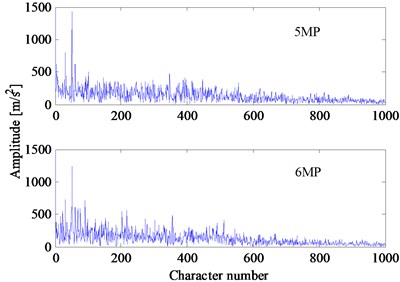
a) Normal

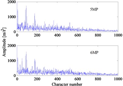
b) Inner race fault

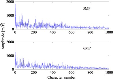
c) Rrolling element fault

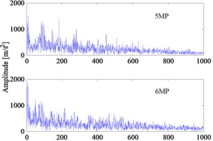
d) multiple faults (inner race fault and rolling element fault)

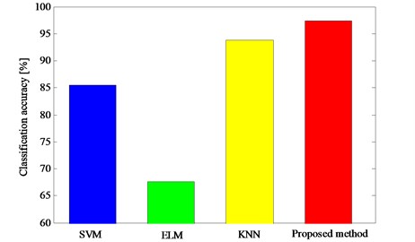
With the increase in the number of hidden units, the DBN classifier model can learn the high complexity non-linear relationships between the input data and the bearing fault types more effectively. In general, the training accuracies and testing accuracies increase if the DBN classifier model has more hidden units. The results in Table 5 demonstrate that the proposed method achieve a high degree of classification accuracy for bearing fault diagnosis. Three classifiers including KNN, SVM, ELM are used for comparison experiment. The parameters of these classifiers are the same as that used in Experiment 1. The results of these classifiers in Fig. 9 verify the superior performance of the proposed method.

Table 4The description of the bearing data set in Experiment 2

Fault type	Training samples	Testing samples	Classification label
Normal	50	50	1
Inner race	50	50	2
Rolling element	50	50	3
Multiple faults	50	50	4

Table 5The classification results of the DBN classifier model in experiment 2

Number of hidden units	Training accuracy (%)	Testing accuracy (%)
10	90.07	85.45
20	96.85	90.26
30	98.14	91.73
40	98.56	94.01
50	100	95.70
60	100	96.22
70	100	95.95
80	100	96.37
90	100	97.09
100	100	97.35

Fig. 9The classification results obtained by different classifier models in experiment 2

5. Conclusions

In this study, a new bearing fault diagnosis method based on Hilbert envelope spectrum and deep belief network is presented. The results in two different experiments fully demonstrate the superior performance of the proposed fault diagnosis method. From the experimental results, it can be concluded as follows:

1) When fault occurs in bearing, the Hilbert envelope spectrum of vibration signal would change and it contains a considerable amount of fault information which can reflect the actual work condition and the fault type of bearing. The Hilbert envelope spectrum of vibration signal can be directly used as eigenvector to express the failure feature of bearing. To reduce the influence of different test conditions on the Hilbert envelope spectrum and make the feature vector more robust, all the vibration signals are firstly resampled in this study. The proposed feature extraction method can avoid complex feature extraction and feature selection.

2) The DBN classifier model is very efficient to learn the high complexity non-linear relationships between high dimension input data (the Hilbert envelope spectrum) and the bearing fault types. The DBN classifier model can be used as both an automatic feature extractor and a classifier for bearing fault diagnosis. Therefore, the bearing fault diagnosis process can be greatly simplified in this study. The DBN classifier model outperforms the traditional classifier such as KNN, SVM and ELM. In sum, the proposed bearing fault diagnosis method based on Hilbert envelope spectrum and deep belief network is not very complex and it can obtain a more excellent diagnostic performance.

References

Li X., Zheng A. N., Zhang X., Li C. C., Zhang L. Rolling element bearing fault detection using support vector machine with improved ant colony optimization. Measurement, Vol. 46, Issue 8, 2013, p. 2726-2734.

Search CrossRef
Zhang P., Du Y., Habetler T. G., Lu B. A survey of condition monitoring and protection methods for medium voltage induction motors. IEEE Transactions on Industry Application, Vol. 47, Issue 2, 2011, p. 34-46.

Search CrossRef
Zhu H. J., Wang X. Q., Zhao Y. Sparse representation based on adaptive multi scale features for robust machinery fault diagnosis. Proceedings of the Institution of Mechanical Engineers, Part C: Journal of Mechanical Engineering Science, 2014.

Search CrossRef
Feng Z. P., Liang M., Chu F. L. Recent advances in time-frequency analysis methods for machinery fault diagnosis: a review with application examples. Mechanical Systems and Signal Processing, Vol. 38, Issue 1, 2013, p. 401-421.

Search CrossRef
Du W. L., Tao J. F., Li Y.M., Liu C. L. Wavelet leaders multi-fractal features based fault diagnosis of rotating mechanism. Mechanical Systems and Signal Processing, Vol. 43, Issue 1-2, 2014, p. 57-75.

Search CrossRef
Yu D. J., Cheng J. S., Yang Y. Application of EMD method and Hilbert spectrum to the fault diagnosis of roller bearings. Mechanical Systems and Signal Processing, Vol. 19, Issue 2, 2005, p. 259-270.

Search CrossRef
Lei Y. G., Lin J., He Z. J., Zuo M. J. A review on empirical mode decomposition in fault diagnosis of rotating machinery. Mechanical Systems and Signal Processing, Vol. 35, Issue 1-2, 2013, p. 108-126.

Search CrossRef
Dong Y. B., Liao M. F., Zhang X. L., Wang F. Z. Faults diagnosis of rolling element bearings based on modified morphological method. Mechanical Systems and Signal Processing, Vol. 25, Issue 4, 2011, p. 1276-1286.

Search CrossRef
Jiang H. M., Chen J., Dong G. M., Liu T., Chen G. Study on Hankel matrix-based SVD and its application in rolling element bearing fault diagnosis. Mechanical Systems and Signal Processing, Vols. 52-53, 2015, p. 338-359.

Search CrossRef
Zhu X. R., Zhang Y. Y., Zhu Y. S. Bearing performance degradation assessment based on the rough support vector data description. Mechanical Systems and Signal Processing, Vol. 34, Issue 4, 2013, p. 203-217.

Search CrossRef
Liu Z. W., Cao H. R., Chen X. F., He Z. J., Shen Z. J. Multi-fault classification based on wavelet SVM with PSO algorithm to analyze vibration signals from rolling element bearings. Neurocomputing, Vol. 99, Issue 1, 2013, p. 399-410.

Search CrossRef
Sun W., Chen J., Li J. Decision tree and PCA-based fault diagnosis of rotating machinery. Mechanical Systems and Signal Processing, Vol. 21, Issue 3, 2007, p. 1300-1317.

Search CrossRef
Saimurugan M., Ramachandran K. I., Sugumaran V., Sakthivel N. R. Multi component fault diagnosis of rotational mechanical system based on decision tree and support vector machine. Expert Systems with Applications, Vol. 38, Issue 4, 2011, p. 3819-3926.

Search CrossRef
Lei Y. G., He Z. J., Zi Y. Y., Chen X. F. New clustering algorithm-based fault diagnosis using compensation distance evaluation technique. Mechanical Systems and Signal Processing, Vol. 22, Issue 2, 2008, p. 419-435.

Search CrossRef
Xu Z. B., Xuan J. P., Shi T. L., Wu B., Hu Y. M. A novel fault diagnosis method of bearing based on improved fuzzy ARTMAP and modified distance discriminant technique. Expert Systems with Applications, Vol. 36, Issue 9, 2009, p. 11801-11807.

Search CrossRef
Samanta B., Al-Balushi K. R. Artificial neural network based fault diagnostics of rolling element bearing using time domain features. Mechanical Systems and Signal Processing, Vol. 17, Issue 2, 2003, p. 317-328.

Search CrossRef
Gryllias K. C., Antoniadis I. A. A support vector machine approach based on physical model training for rolling element bearing fault detection in industrial environments. Engineering Application and Artificial Intelligent, Vol. 25, Issue 2, 2012, p. 326-344.

Search CrossRef
Hinton G. E., Salakhutdinov R. R. Reducing the dimensionality of data with neural networks. Science, Vol. 313, Issue 5786, 2006, p. 504-507.

Search CrossRef
Bengio Y. Learning deep architectures for AI. Foundations and Trends in Machine Learning, Vol. 21, Issue 6, 2009, p. 1601-1621.

Search CrossRef
Kuremoto K., Kimura S., Kobayashi K., Obayashi M. Time series forecasting using a deep belief network with restricted Boltzmann machines. Neurocomputing, Vol. 137, Issue 5, 2014, p. 47-56.

Search CrossRef
Shang C., Yang F., Huang D. X., Lyu W. X. Data-driven soft sensor development based on deep learning technique. Journal of Process Control, Vol. 24, Issue 2, 2014, p. 223-233.

Search CrossRef
Tran V. T., AlThobiani F., Ball A. An approach to fault diagnosis of reciprocating compressor valves using Teager–Kaiser energy operator and deep belief networks. Expert Systems with Application, Vol. 41, Issue 9, 2014, p. 4113-4122.

Search CrossRef
Fisher A., Igel C. Training restricted Boltzmann machines: an introduction. Pattern Recognition, Vol. 47, Issue 1, 2014, p. 25-39.

Search CrossRef
Hinton G. E. A practical guide to training restricted Boltzmann machines. Momentum, Vol. 9, Issue 1, 2010, p. 1-21.

Search CrossRef
Loparo K. A. Bearing data set. Case Western Reserve University Bearing Data Center. http://www.eecs.case.edu/laboratory/bearing/download.htm.

Search CrossRef
Hu Q., He Z. J., Zhang Z. S., Zi Y. Y. Fault diagnosis of rotating machinery based on improved wavelet package transform and SVMs ensemble. Mechanical Systems and Signal Processing, Vol. 21, Issue 2, 2007, p. 688-705.

Search CrossRef
Lei Y. G., He Z. J., Zi Y. Y., Hu Q. Fault diagnosis of rotating machinery based on multiple ANFIS combination with GAs. Mechanical Systems and Signal Processing, Vol. 21, Issue 5, 2007, p. 2280-2294.

Search CrossRef
Du J., Wang S. P., Zhang H. Y. Layered clustering multi-fault diagnosis for hydraulic piston pump. Mechanical Systems and Signal Processing, Vol. 36, Issue 2, 2013, p. 487-504.

Search CrossRef

About this article

Received

12 January 2015

Accepted

11 April 2015

Published

15 May 2015

SUBJECTS

Fault diagnosis based on vibration signal analysis

Keywords

bearing fault diagnosis

statistical feature

Hilbert envelope spectrum

deep belief network

This is an open access article distributed under the Creative Commons Attribution License, which permits unrestricted use, distribution, and reproduction in any medium, provided the original work is properly cited.