An intelligent fault diagnosis method using variable weight artificial immune recognizers (V-AIR)

Zhang, Hongli; Liu, Jicheng; Zhou, Erping; Li, Dong; Wang, Bo; Shi, Kunju

Journal of Vibroengineering

Browse Journal

Submit article

Published: 15 August 2015

Check for updates

An intelligent fault diagnosis method using variable weight artificial immune recognizers (V-AIR)

Hongli Zhang¹

Jicheng Liu²

Erping Zhou³

Dong Li⁴

Bo Wang⁵

Kunju Shi⁶

¹Shanghai Institute of Applied Mathematics and Mechanics, Shanghai University, Shanghai 20072, China

^{1, 2, 4, 5, 6}School of Mechatronics Engineering and Automation, Shanghai University, Shanghai 200072, China

³University of Bolton, Bolton, UK

Corresponding Author:

Jicheng Liu

Cite the article Download PDF

Downloads 1119

Abstract

The Artificial Immune Recognition System (AIRS), which has been proved to be a successful classification method in the field of Artificial Immune Systems, has been used in many classification problems and gained good classification effect. However, the network inhibition mechanisms used in these methods are based on the threshold inhibition and the cells with low affinity will be deleted directly from the network, which will misrepresent the key features of the data set for not considering the density information within the data. In this paper, we utilize the concept of data potential field and propose a new weight optimizing network inhibition algorithm called variable weight artificial immune recognizer (V-AIR) where we replace the network inhibiting mechanism based on affinity with the inhibiting mechanism based on weight optimizing. The concept of data potential field was also used to describe the data distribution around training samples and the pattern of a training data belongs to the class with the largest potential field. At last, we used this algorithm to rolling bearing analog fault diagnosis and reciprocating compressor valves fault diagnosis, which get a good classification effect.

1. Introduction

Immune system has been noticed by many computer sciences and engineering researchers, for it has many advantages that many artificial-intelligence systems can’t match such as the distinction of self-nonself molecules, early warning of danger signals, distributed disposition of hazardous situations and incremental learning. Thus, the immune system characteristics has been developed and applied in many engineering field [1]. In the last decade, several interdisciplinary research scientists have produced a prolific amount of immune inspired algorithms, mathematical models and hybrid intelligent systems by extracting one or more properties, function and mechanism of immune system.

Based on the principles of self-nonself discrimination of immune system, one of the major algorithms developed is the Negative Selection Algorithm (NSA) which is analogous to the censoring process of T cell maturation in immune system [2, 3]. The NSA generates detectors randomly and eliminates the ones that detect self so that the remaining detectors can detect any non-self [4]. Since the matching criterion is not specific, we can cover the non-self space with limited number of detectors. However, the original NSA represents detectors in binary, which may not capture the structure of some problem spaces or cause a low level of computing efficiency [5]. The real-valued negative selection (RNS) extends the previous binary anomaly detectors to real space anomaly detectors [5, 6] and a lot of further researches concentrating on detector generation schemes also have sprung up such as the hyper-rectangular detectors [5], the variable-sized detectors (V-detector) [7, 8], the hyper-ellipsoid detector [9]. Nevertheless, almost all of the methods don’t consider the distribution density of self samples and use constant-size self hyperspheres to express the profile of self space, which may increase false alarm rates with a smaller self radius and decreases detection rates on the contrary. The ANSA disposes the issue with variable-sized self radius and acquires a great of achievement [10].

Another method of imitating the immune system is to use the specific immunity of B cells. Compared with NSA, it is a straightforward artificial immune algorithm and called as “positive selection algorithm”. Jerne [11] and Farmer [12] firstly proposed the immune network theory to illustrate the B cell concentration changes. Inspired by the immune network theory, a clustering algorithms-ainet model was firstly invented to find some memory points called as memory antibodies representing the data distribution. As an information compression algorithm, the algorithm can largely reduce the number of memory cells, however, it also may misrepresent the key features of the data for not considering the density information within the data [13, 14]. So the Adaptive Radius Immune Algorithm (ARIA) [15] introduces an antibody adaptive suppression radius that varies inversely with the local density for each antibody’s neighborhood to preserve the density information of the data set and obtains a superior performance.

Artificial immune network model (AINE) is another algorithm obtained by the proposing of B cell stimulation and network affinity threshold [16]. The most successful unsupervised learning algorithm based on AINE is the resource limited artificial immune system (RLAIS) which not only uses the immune network dynamics and introduces the concept of shape-space but also puts forward the concept of artificial recognition ball (ARB) [17]. Influenced by the concept of ARB in RLAIS, Watkins et al. [18] put forward a supervised learning algorithm named as Artificial Immune Recognition System (AIRS) using the immune mechanism of high frequency variation, clonal mutation, resource allocation mechanism and network suppression. Since then, AIRS is applied to a serial of classification problems and a lot of improved algorithms continuously emerge. A hybrid classifier that uses the fuzzy weighted pre-processing to weight the input data and the AIRS classifier shows an effective performance on several problems such as machine learning benchmark problems and medical classification problems [19, 20]. In the study of Polat et al. [21], a new resource allocation mechanism was done with fuzzy-logic in the Fuzzy-AIRS. As a further research, another nonlinear recognition system involving AIS and ANN (artificial neural network (ANN)-aided AIS-response, AaA-response) was proposed, which used multiple antibodies to form an output for a presented input [22]. In the research of MAIRS2, a modified AIRS2 was used to replace the $k$ -nearest neighbor algorithm with the fuzzy $k$ -nearest neighbor to improve the diagnostic accuracy of diabetes diseases. However, the network inhibition mechanisms used in these methods are all based on threshold inhibition and the cells with low affinity will be deleted directly from the network, so as an information compression algorithm it may misrepresent the key features of the data set for the relative distances among the trained memory cells did not adequately represent the original data [13-15].

In this paper, we utilize the concept of data potential field and propose a new classification method called variable weight artificial immune recognizers (V-AIR). In this algorithm, we use weight optimizing inhibition mechanism to realize the network inhibition mechanism, which is realized by quadratic programming. In this way, for high density portion of training samples, memory cells are allowed to have larger weights; for sparse region of samples, the memory cells are allowed to have smaller weights. Therefore, this method reflects the density distribution information of data through increasing the memory cell’s weight in dense region and decreasing the weight of memory cells in sparse region. In testing phase, the pattern of a training data belongs to the class with the largest potential field.

This paper is structured as follows: In the next section, we give our motivation to the definition of data potential field. In Section 3, we introduce the V-AIR to solve the problem of data classification. Related works are also discussed in Section 3. In Section 4, 4 kinds UCI data sets are used to compare with AIRS. Beside, rolling bearing fault diagnosis is also researched to prove the effectiveness of V-AIR.

2. Definition of data potential field

In 1837, British physicist Faraday firstly proposed the concept of physical to describe the non-contact effect among objects. He thought the occurrence of non-contact interaction such as the universal gravitation, electrostatic force and magnetic force must be achieved with some intermediate medium and the medium is field. With the development of field theory, people abstracted this as a mathematical concept [23]:

Definition 1: If every point in the space corresponds to a certain physical or mathematical value, a field can be determined in the space and this field can be expressed with different univalent functions according to different objects such as:

- The gravitational field:

1

φ (r) = G \times \sum_{i = 1}^{n} \frac{m_{i}}{‖r - r_{i}‖},

with $m_{i}$ is the weight of a particle, $‖r - r_{i}‖$ is distance between site $r$ and particle $r_{i}$ ;

- The nuclear field:

2

φ (r) = V_{0} \times e^{- {(\frac{‖r - r_{i}‖}{R})}^{2}},

with $V_{i}$ is the weight of a nucleus, $‖r - r_{i}‖$ is the distance between site $r$ and nucleus $r_{i}$ , $R$ is the scope of nuclear force.

Referencing the thought of field in physics, Li et al. [23] also introduced the concept of potential field into the number field space and created the data potential field:

Definition 2: Given a data set with $N$ objects $D = {x_{1}, x_{2}, \dots, x_{n}}$ in space $Ω \subseteq R^{p}$ . A field can be determined in the space and this field can be expressed with different univalent functions according to different objects such as:

3

φ (x) = \sum_{i = 1}^{N} φ_{i} (x) = \sum_{i = 1}^{N} m_{i} \times e^{- {(\frac{‖x - x_{i}‖}{δ})}^{2}},

with $‖ x - x_{i} ‖$ is the distance between site $x$ and nucleus $x_{i}$ , $m_{i}$ is the weight of nucleus $x_{i}$ , $δ$ is the impact factor of nuclear field function. Assuming that the normalization condition meet, we have:

4

\sum_{i = 1}^{n} m_{i} = 1 .

Similar to the contour in physics, we also represent the characteristics of physical field distribution with the potential function.

3. The variable weight artificial immune recognizers (V-AIR)

In this research, an innovative classification model called variable weight artificial immune recognizers (V-AIR) is proposed. The motivation for developing this algorithm comes from the fact that deleting an antibody from the immune system directly may misrepresent the key features of data set for not considering the density information within the data. In this paper, we utilize the concept of potential field data and propose a new weight optimizing network inhibition algorithm called variable weight artificial immune recognizers (V-AIR) where we replace the network inhibiting mechanism based on affinity with the inhibiting mechanism based on weight optimizing. In this algorithm, the weights of memory cells are optimized by the quadratic programming and the cells with weights below the setting threshold will be deleted directly from the memory network. In this way, for high density portion of training samples, memory cells are allowed to have a larger weight; for sparse region of samples, memory cells are allowed to have a smaller weight. Therefore, this method reflects the density distribution information of data through increasing the memory cell’s weight in dense region and decreasing the weight of memory cells in sparse region. To describe conveniently, V-AIR also introduces the concept of Artificial Recognition Ball (ARB) and variable weight memory cells ( $V$ - $m c$ ). Like the memory cells used in RLAIS and AIRS [17, 18], a $V$ - $m c$ also represents a number of identical B cells but has a variable weight changing according to the result of optimizing.

3.1. The algorithm description

The V-AIR can be described specifically as follows:

$A G_{h}$ : the antigen set of $h$ th class, $A G_{h} \in R^{M \times L}$ . L is the dimension of attributive character, $M$ is the number of antigens belonging to a class.

$M C$ - $P_{h}$ : the memory cell pool used for the $h$ class antigens, which represents the collection of memory cells, $M C \in R^{N \times L}$ . $L$ is the dimension of attributive character, $N$ is the number of memory cells.

$A g_{h i}$ : the $i$ th antigen belonging to $h$ class, $A g_{h i} \in A G_{h}$ .

$A R B$ - $P_{h}$ : the artificial recognition ball pool used for $h$ th antigens. It is used for storing the cells produced in the process of cloning.

$A R B_{h j}$ : stored in $A R B$ - $P_{h}$ and corresponds to the $j$ th ARB of class $h$ , $A R B_{h j} \in A R B - P_{h}$ .

$C$ - $m c_{h i}$ : the $i$ th candidate memory cells stored in $M C$ - $P_{h}$ , $C - m c_{h i} \in M C - P_{h}$ .

$V$ - $m c_{h i}$ : the retained memory cells after quadratic programming, which is also stored in $M C$ - $P_{h}$ with a variable weight.

$A f$ : the measure of similarity degree or affinity between antigen and antibody cells, the value in V-AIR is expressed with kernel function, such as:

5

A f (V - A R {B_{h}}_{j}, A g_{h i}) = e^{- {(\frac{‖V - A R B_{h j} (j, :) - A g_{h i} (i, :)‖}{δ})}^{2}},

where $R e_{h}$ : the $V - A R B_{h}$ ’s total resources, $N_{h j}$ : the clone scales of $A R B_{h j}$ , $T$ : the cloning coefficient of $A R B_{h}$ , $M_{r}$ : the mutation rate of $A R B_{h}$ , $s_{h}$ : the average affinity threshold between antigen and ARB, $C_{h}$ : the number of class $h$ ’s ARBbefore resource allocation, $C_{h}^{*}$ : the number of $A R B_{h}$ ’s after resource allocation, $R_{s}$ : the total number of resource that all $A R B_{h}$ are allowed to have, $δ$ : the impact factor of nuclear field function, $r$ : the variable coefficient to adjust the merging criteria between antibodies, $D$ : the number of antigen categories, $E_{t}$ : the setting threshold to delete or reserve an $V$ - $m c$ . If the weight of an $V$ - $m c$ is greater than $E_{t}$ , the $V$ - $m c$ will be reserved. If the weight of an $V$ - $m c$ is smaller than $E_{t}$ , the $V$ - $m c$ will be deleted.

During the training process, all kinds of antigens are independent of each other, so we can freely take the antigens of class $h$ as the instance to illustrate the generative process of $V$ - $m c$ . The following of this part will instruct the steps of the algorithm in detail:

1. Initialization: In this part, we firstly normalize the training samples in the unit square ${[0, 1]}^{n}$ . At the same time, the required input: $A G_{h}$ , $s_{h}$ , $R_{s}$ , $δ$ , $r$ , $T$ , $E_{t}$ , $k$ are also set. The initial $A R B_{h} s$ in $A R B$ - $P_{h}$ are generated randomly on this step.

2. The produce of candidate memory cells: For every $A g_{h i}$ ( $i =$ 1, 2, …, $M$ ), do the following steps:

a) Calculate the affinity $A f$ between $A g_{h i}$ and the initialized $A R B_{h} s$ .

b) Clone and mutate $A R B_{h j}$ with $N_{h j} = T^{*} A_{f} (A R B_{h j}, A g_{h i})$ and mutation rate $M_{r}$ . Then get the number of $A R B_{h} s$ , which are labeled as $C_{h}$ .

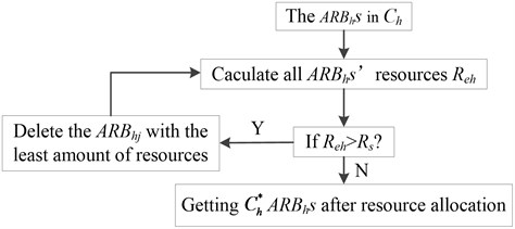
c) Calculate the total $A R B_{h}$ s’ resources $R_{e h} = \sum_{j = 1}^{C_{h}} N_{h j}$ and distribute the resource in $A R B_{h} s$ , until the $R_{e h} \leq R_{s}$ . This will result in some $A R B_{h} s$ with resource approaching 0 to die and ultimately control the population. The specific process of resource allocation is shown in Fig. 1.

d) Calculate the average affinity $A f$ between $A R B_{h} s$ and $A g_{h i}$ , if the average affinity $A f$ larger than $s_{h}$ , select the candidate memory cells ( $C$ - $m c_{h} s$ ); if the average affinity $A f$ less than $s_{h}$ , return to step (b) until meeting the affinity conditions.

e) Choose the $A R B_{h j}$ with highest affinity and take it as a $C$ - $m c_{h i}$ . The $C$ - $m c_{h i}$ will be put into $M C$ - $P_{h}$ .

The step (a)-(e) will be looped until all of the class $h$ antigens are processed.

Fig. 1The process of resource allocation

3. The network inhibition of candidate memory cells: The weights of $C$ - $m c_{h} s$ in $M C$ - $P_{h}$ (or the concentration of each $C$ - $m c_{h i}$ ) are optimized by quadratic programming function and the $C$ - $m c_{h} s$ with weight below the setting threshold $E_{r}$ will be deleted directly from the memory network. At last, the retained $C$ - $m c_{h} s$ change into $V$ - $m c_{h} s$ and constitute the $M C$ - $P_{h}$ .

After all the $D$ types of training antigens are recognized, the $V$ - $m c_{h} s$ will be used for data classification. The classification process is conducted by the principle of potential field dominant namely each kind of $V$ - $m c_{h} s$ ’ potential field is superposed at the point of the test sample $Y_{k}$ , which can get the potential field value of $Y_{k}$ belonging to each kind of $V$ - $m c_{h}$ : $φ_{1}$ , $φ_{2}$ , …, $φ_{D}$ and $Y_{k}$ belongs to the class with the largest superimposed potential field $φ_{i}$ .

As a supervised learning classification system, each antigen $A g_{h i}$ has its class and produces many $A R B_{h} s$ responding to this antigen $A g_{h i}$ . After clone mutation and resource allocation process, the $A R B_{h} s$ with resource equal to 0 will be deleted from the $A R B$ - $P_{h}$ directly. The $A R B_{h} s$ with the strongest response will be seen as the $C$ - $m c_{h} s$ and put into the $M C$ - $P_{h}$ . However, the number of these $C$ - $m c_{h} s$ still exceeds the people’s cognitive needs, so we need to use the quadratic programming function to estimate the weights of objects and get a few non-zero core objects to reduce the number of memory cells. At last, the several core objects are used to represent the data classification model. The quadratic simplified estimation process is as follows: In $Ω \in R^{d}$ , the set of $H = \{C - m c_{h 1}, C - m c_{h 2}, \dots, C - m c_{h E}\}$ includes $E$ candidate memory cells. Besides, in order to describe conveniently, we describe them as $H = \{X_{1}, X_{2}, \dots, X_{E}\}$ , so according to the concept of data potential field, the data potential field of any test sample in the space can be decided as:

6

φ (Y) = \sum_{i = 1}^{E} φ_{i} (Y) = \sum_{i = 1}^{E} (m_{i} \times e^{- {(\frac{‖Y - X_{i}‖}{δ})}^{2}}) .

When the weights of objects don’t require equal, the weight of $m_{1}$ , $m_{2}$ ,…, $m_{E}$ can be seen as a group of function according to spatial position $X_{1}$ , $X_{2}$ ,…, $X_{E}$ . If the population distribution is known, the weights of all objects can be estimated through minimizing the error criterion between potential function $φ (Y)$ and distribution density function. Assuming that the overall density of all objects is $p (Y)$ , so when the value of $δ$ is certain, we can minimize the following integral square error criterion [24]:

7

m i n J = \underset{{m_{i}}}{m i n} \int_{Ω} {[\frac{φ (Y)}{{(\sqrt{π} σ)}^{d}} - p (Y)]}^{2} d x .

Accessibility:

8

m i n J = \underset{{m_{i}}}{m i n} \int_{Ω} [\frac{φ^{2} (Y)}{{(\sqrt{π} σ)}^{2 d}} - \frac{2 p (Y) \cdot φ (Y)}{{(\sqrt{π} σ)}^{d}} + p^{2} (Y)] d x .

Obviously, $\int_{Ω} p^{2} (Y) d x$ has nothing to do with $m_{1}$ , $m_{2}$ ,…, $m_{E}$ , so the objective function can be simplified as:

9

m i n J = \underset{{m_{i}}}{m i n} [\int_{Ω} \frac{φ^{2} (Y)}{2 {(\sqrt{π} σ)}^{d}} d x - \int_{Ω} p (Y) φ (Y) d x] .

Analysis the following function, $\int_{Ω} p (Y) φ (Y) d x$ is the mathematical expectation of $φ (Y)$ and we can use $E$ independent extraction samples to approximate:

10

m i n J = \underset{{m_{i}}}{m i n} [\frac{1}{2 {(\sqrt{π} σ)}^{d}} \int_{Ω} φ^{2} (Y) d x - \frac{1}{E} \sum_{j}^{E} φ (X_{j})],

with Eq. (5), can get:

11

m i n J = \underset{{m_{i}}}{m i n} [\frac{1}{2 {(\sqrt{2})}^{d}} \sum_{i = 1}^{E} \sum_{j = 1}^{E} m_{i} \times m_{j} \times e^{- {(\frac{‖Y_{i} - Y_{j}‖}{\sqrt{2} δ})}^{2}} - \frac{1}{E} \sum_{i = 1}^{E} \sum_{j = 1}^{E} m_{i} \times e^{- {(\frac{‖Y_{i} - Y_{j}‖}{δ})}^{2}}] .

Obviously, this is a typical constrained quadratic programming problem and satisfies the following constraint conditions:

12

\sum_{i = 1}^{E} m_{i} = 1,

with $m_{i} \geq 0$ .

Optimize the Eq. (11) and get a set of optimal weights. The optimization result is a few objects in the candidate memory cell concentration areas having great weights and most objects with much smaller weights or a weight of zero.

4. Combining mutation: After each presentation of the training antigen, the $V$ - $m c_{h i} s$ are generated with the variable weights calculated by Eq. (11). However, these cells still have large coincidence with each other for each training antigen being assigned a $V$ - $m c_{h i}$ , which increases the computational complexity. Thus, the redundant $V$ - $m c_{h i}$ must be cleared away. However, if an antibody is deleted from the memory antibody network directly, the rest memory antibody would be far away from the antigen and cause the relative distances distortion phenomenon between memory antibodies. So, in this paper we decrease the coincidence and reduce the number of them through merge the similar two memory cells into a new one. We call this merger as combining mutation for the position and weight of the memory cells changed.

When the distance between two memory cells satisfies the inequality, the two memory cells can be merged into a new one:

13

‖Y_{i} - Y_{j}‖ \leq r \times δ \times (M_{i} + M_{j}),

where $r$ is a variable coefficient to adjust the merging criteria between the antibodies, $Y_{i}$ and $Y_{j}$ are the spatial position of the original two memory cells. Here we use the momentum conservation law [23] as the merge mutation rule and the fusion memory cell’s new position and weight can be calculated by the following equation:

14

Y_{n e w} = \frac{M_{i} \times Y_{i} + M_{j} \times Y_{j}}{M_{i} + M_{j}}, (i \neq j),

15

M_{n e w} = M_{i} + M_{j} (i \neq j),

where $Y_{n e w}$ is the new spatial position of fusion memory cell, $M_{i}$ and $M_{j}$ are the weights of memory cells to be merged, $Y_{i}$ and $Y_{j}$ are the spatial position of the original two memory cells and $M_{n e w}$ is the new weight of fusion memory cell. The merging mutation is recursively implemented, until all the memory cells that meet the merging condition are merged. Through multiple combining mutations, some fusion memory cell would claim a larger and larger weight calculated by Eq. (15). From Eq. (14), we also find that the fusion memory cell would get more close to the center of larger weight memory cell and the larger weight the memory cell have, the closer the fusion memory cell will be. Thus, through many times combining mutation, some fusion memory cells would have much larger weights than other memory cells needed to be merged. In the extreme cases, if the other memory cell’s weight is too small to be ignored, the weight and spatial position of the fusion memory cell will have no change in the combining mutation.

5. Recognition phase: After training has completed, each $V$ - $m c_{h i}$ in $M C$ is endowed with a weight. In view of the unbalance factor of the training samples, a $V$ - $m c_{h i}$ ’s weight should be divided by the number of the training antigens of its class $j$ , so the weight of $V$ - $m c_{h i}$ is changed into:

16

h_{i} = \frac{m_{i}}{N_{j}},

where $h_{i}$ is the weight of $V$ - $m c_{h i}$ after transformation, $m_{i}$ is the weight of $V$ - $m c_{h i}$ before transformation and $N_{j}$ is the number of training samples of class $j$ . The affinity between a test antigen and a $V$ - $m c_{h i}$ changes from Eq. (3) into:

17

a f f i n i t y (Y, X_{t}) = h_{i} \times e^{- {(\frac{‖Y - X_{t}‖}{δ})}^{2}} .

In the next, the recognition phase is performed in a new nearest neighbor approach: $k$ - weight nearest neighbor approach. Like the $k$ -nearest neighbor approach, this method firstly presents each test sample to all of the memory cells and then picks out the $k$ memory cells with the largest affinities in $M C$ . However, the system’s classification of a data item is not determined directly by using a majority vote of the outputs of the $k$ most nearest memory cells. In our $k$ -weight nearest neighbor approach, the minimum affinity memory cell is endowed with a vote of 1 and the votes for the $k$ most nearest memory cells are decided by the following equation:

18

V_{i} = \frac{a f f i n i t y (Y, X_{i})}{m i n (a f f i n i t y (Y, X_{1}), a f f i n i t y (Y, X_{2}), \dots, a f f i n i t y (Y, X_{k}))},

where $V_{i}$ is the vote for test antigen $Y$ . So the memory cell’s vote for a test antigen is converted into decimals and the classification of the test antigen belongs to the class with the largest total value of votes, e.g. in the 3-weight nearest neighbor approach, for a test antigen if there are two nearest memory cells in class 1 with the votes $V_{1} =$ 1, $V_{2} =$ 1.1 and one nearest memory cell in class 2 with the vote $V_{3} =$ 2.2, then the test sample belongs to the class 2 not the class 1.

3.2. The flow of V-AIR algorithm

V-AIR uses the quadratic to imitate the network inhibition mechanism among $V$ - $m c s$ and distribute the number of B cells included in a $V$ - $m c$ . Like the the method used in AIRS, the antigens used in V-AIR are firstly initialized as eigenvectors $A g_{i} = (x_{i 1}, x_{i 2}, \dots, x_{i n})$ and proposed to the system during training and learning process. The B cells are also expressed as eigenvectors $A b_{i} = (y_{i 1}, y_{i 2}, \dots, y_{i n})$ with $x_{i k}$ and $y_{i k}$ $(k =$ 1, 2,…, $n)$ expressing the $i th$ attributive character of $A g_{i}$ or $A b_{j}$ respectively. To reduce the repetition of B cells, the same B cells are expressed as a ARB and the memory cell are expressed as a $V$ - $m c$ . The key of the algorithm is to use the mechanism of quadratic programming optimizing the weight of $V$ - $m c$ and use the data field to classify the testing data.

Fig. 2The flow diagram of V-AIR

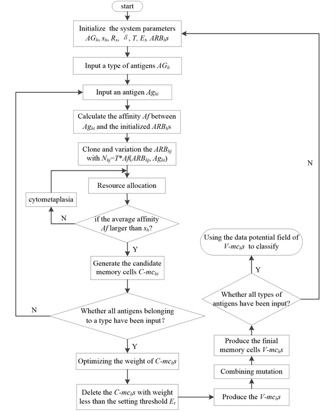
In general, the V-AIR can be divided into two stages: the limited resource competition stage and the quadratic programming phase of $C$ - $m c_{h} s$ . The limited resource competition stage mainly uses the clone variation and limited resources allocation mechanism to imitate the somatic hyper mutation, clone suppression and immune homeostasis process in human immune system. In the human immune system, there is also network suppression among B cells: when the external antigens invade, some B cells in the immune system will clone and amplify and its concentration would increase; however, some other B cells will die and its concentration would decrease. In V-AIR, we use the quadratic programming to achieve this function. Fig. 2 gives the description of this algorithm.

4. Application of V-AIR to classification

This section briefly touched on the effect of parameters and some comparisons between the existing techniques presented in [18]. The focus of parameters’ discussion was mainly on two of the important features of V-AIR algorithms: classification accuracy and memory cell reduction. In the comparisons, experiments were carried out using four UCI datasets [25]: the Fisher Iris, Pima diabetes, Ionosphere and Sonar data sets.

4.1. Classification accuracy

In this study, the classification accuracies for the datasets were measured according to Eq. (19) [20, 21]:

19

a c c u r a c y (T) = \frac{\sum_{j = 1}^{T} a s s e s s (Y_{i})}{T}, Y_{i} \in T,

a s s e s s (Y) = \{\begin{array}{l} 1, if c l a s s i f y (Y) = Y . c, \\ 0, otherwise, \end{array}

where $T$ is the set of data items to be classified (the test set), $Y . c$ is the class of the item $Y$ , and classify $Y$ returns the classification of $Y$ by V-AIR or AIRS.

4.2. Effect of parameters

V-AIR is a multi-parameter classification system, so it is important to evaluate that the behavior of V-AIR is altered with respect to the user defined parameters in actual engineering. In order to establish this, investigations were undertaken to determine what affect two of the most important features: the number of memory cells and the classification accuracy. For V-AIR has 8 parameters to analyze, so the effect of each parameter is analyzed to determine which one is more likely to affect the above two items.

In the V-AIR classification method, once a set of memory cells has been developed, the resultant cells can be used for classification. As described in 3.1, obviously we can conclude that the mutation rate $M_{r}$ , clonal rate $T$ and number of resource $R_{s}$ allowed in V-AIR only associate with the evolution speed of $A R B_{h}$ but have nothing to do with the classification accuracy. Thus, in the analysis of classification accuracy and number of memory cells, we need not to consider the 3 parameters. The average stimulation threshold $s_{h}$ is an evaluation parameter to determine the degree of affinity between antigens and antibodies. In the process of clonal variation, if $s_{h}$ is set too large, $A R B_{h}$ would spend more time to cycle the clone and mutation process until the termination condition satisfied; if $s_{h}$ is set too small, $A R B_{h}$ would have small affinity with the target antigen $A g_{h i}$ which can affect the classification accuracy in some degree. Therefore, $s_{h}$ should be set in a suitable range. According to Eq. (5), $s_{h}$ is a parameter changing in (0, 1], so we give the instructional scope between 0.6 and 0.94. The setting threshold $E_{t}$ , which also changes between 0 and 1, determines the number of reserved $C$ - $m c_{h} s$ and can affect the number of memory cells and classification accuracy in some degree. Because when $E_{t}$ is set large, less $C$ - $m c_{h} s$ are used for generating $V$ - $m c_{h} s$ . Meanwhile the classification accuracy and number of memory cells are both reduced in some degree. When $E_{t}$ is set small, more $C$ - $m c_{h} s$ are used for generating $V$ - $m c_{h} s$ which increase the number of memory cells. The classification accuracy would also be affected in some extent for more $C$ - $m c_{h} s$ are reserved to produce the $V$ - $m c_{h} s$ . However, according to Eq. (5), when $E_{t}$ is little enough, the reserved $V$ - $m c_{h}$ with small weight would have little influence to final data classification for the $A f$ calculated by Eq. (5) can be ignored. Hence, we give the guidance value of $E_{t} =$ 0.001 at here. The $k$ value of V-AIR determines the number of nearest neighbor used for classification and has nothing to do with the number of memory cells but relates with the classification accuracy. In the process of application, we give the guidance value between 3 to 7 if the number of $V$ - $m c_{h} s$ greater than 3 or use all of the $V$ - $m c_{h} s$ when the number of $V$ - $m c_{h} s$ below 3.

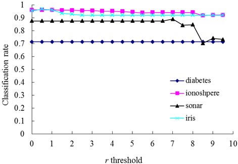
In our method, the number of memory cells and the detection rate are mainly affected by the parameters $r$ and $δ$ . In order to illustrate the varying rules of them, investigations are firstly undertaken with the diabetes, ionosphere, sonar and iris dataset to determine how do the changes of $δ$ and $r$ affect the number of memory cells (Fig. 3 and 5) and the classification accuracy (Figs. 4 and 6).

Fig. 3The change of memory cells with changing values of the δ threshold

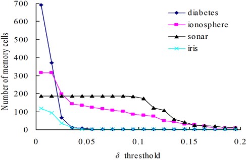
Fig. 4The change of classification rate with changing values of the δ threshold

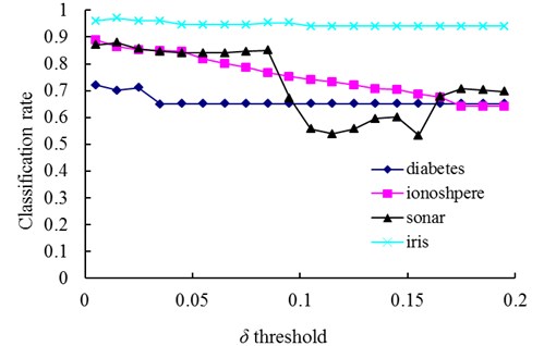
The relationships between the parameter $δ$ and the number of memory cells in V-AIR for the four UCI datasets (Diabetes, Ionosphere, Sonar and Iris dataset) are shown in Fig. 3. The variation tendencies of the classification accuracy following with the parameter $δ$ are also shown in Fig. 4. In Fig. 3, the number of memory cells decreases gradually as the increase of the parameter $δ$ , for more memory cells satisfies the Eq. (5). At last, all of the memory cells belonging to one training class will be combined into one memory cell and the curves for memory cells’ number don’t change again. During the change of the memory cells’ number, the classification accuracy of memory cells also fluctuate significantly but at last, the classification accuracy will becomes calm and steady ultimately, for the number of memory cells never changes again. In Figs. 5-6, altering the parameter $r$ with a fixed parameter $δ$ for each type of datasets, the number of memory cells and the classification accuracy show the same varying patterns with Figs. 3-4.

Fig. 5The change of memory cells with changing values of the r threshold

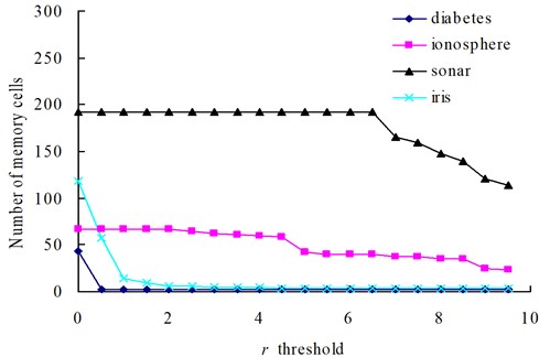
Fig. 6The change of classification rate with changing values of the r threshold

4.3. Comparison of V-AIR with AIRS

To have a stark comparison, we show the performance of V-AIR on these data sets with the results of AIRS [18] in Tables 1-2. The parameters used in V-AIR are set in Table 3. Since AIRS and V-AIR use all the memory cells to classify the unknown data, the classification cost is proportional to the number of cells. Like the method used in [18], these results are also obtained from the averaging multiple runs of V-AIR, typically consisting of three or more runs and five-way, or greater, cross validation. For the Iris date set, a five-fold cross validation scheme is employed with each result representing an average of three runs across these five divisions. For the Ionosphere data set, we remain the division method as detailed in AIRS: 200 instances hic are carefully split almost 50 % positive and 50 % negative are used for training with the remaining 151 as test instances, consisting of 125 “good” and only 26 “bad” instances. The results reported here also represent an average of three runs. For the Diabetes data set a ten-fold cross validation scheme is used, again with each of the 10 testing sets being disjoint from the others and the results are averaged over three runs across these data sets. The Sonar date set is divided randomly into 13 disjoint sets with 16 cases in each. 12 of these sets are used as training data with 1 as the test date.

The accuracy of V-AIR for Iris, Diabetes, Ionosphere and Sonar is about 0.6 %, 0.3 %, 0.7 % and 1.9 % higher than the AIRS’s in Table 1. The accuracy of V-AIR for these four UCI date sets is sufficiently comparable with that of the AIRS classifier but this method requires more memory cells in the classification of Diabetes, Ionosphere and Sonar (Table 2), which means higher computational complexity. However, in the classification of Iris, the V-AIR uses only average of 23.8 memory cells and implements the 97.3 % classification accuracy. Thus, to further validate the advantage of our method, we use it in bearing analog failure with the data set of Case Western Reserve University.

Table 1Comparisons of accuracy between AIRS and V-AIR

Training set	V-AIR: accuracy (%)	AIRS: accuracy (%)
Iris	97.3 (0.1)	96.7 (3.1)
Diabetes	74.5 (0.7)	74.2 (4.4)
Ionosphere	96.3 (0.1)	95.6 (1.7)
Sonar	86.8 (0.1)	84.9 (9.1)

Table 2Comparisons of the average number of memory cells between V-AIR and AIRS. Size refers to the number of training data and the percentage refers to the compression ratio of memory cells

Training set	Size	V-AIR: memory cells	AIRS: memory cells
Iris	120	23.8/81 % (5.6)	30.9/74 % (4.1)
Diabetes	691	691/0 % (0.0)	273.4/60 % (20.0)
Ionosphere	200	169.6/15 % (5.5)	96.3/52 % (5.5)
Sonar	192	189.7/1 % (0.8)	177.7/7 % (4.5)

Table 3Used parameters in V-AIR for UCI datasets

Used parameters	Diabetes	Ionosphere	Sonar	Iris
Mutation rate	0.7	0.7	0.7	0.7
Average stimulation threshold	0.9	0.9	0.9	0.9
Clonal rate	100	100	100	100
Number of resources allowed in V-AIR	40	40	40	40
$k$ value for $k$ -weight nearest neighbor	7	7	3	7
$r$ value	0.705	50	7	0.4
$δ$ value	0.001	0.0015	0.025	0.02
$E_{t}$ value	0.001	0.001	0.001	0.001

5. Application of V-AIR in equipment fault diagnosis

The fault of many equipment usually has the characteristics of complexity and nonlinear. In addition, they also often have small signal noise ratio (SNR) with the weak fault. As a fault simulation instance, the ball bearing data set of Case Western Reserve University [25] was firstly introduced to do the bearing fault diagnosis experiment in this section. Then, as an industrial case, the V-AIR was conducted using the gas valves failure data for piston compressors to validate the feasibility of our failure diagnosis method with the appropriate parameters. The influence of parameters’ change on the classification rate and number of memory cells is also discussed in this section.

5.1. The diagnosis of bearing analog failure

In this paper, three kinds of fault samples are used for verifying the effectiveness of the proposed method. Fig. 7 gives the time domain vibration waveform of rolling bearing in normal state, 0.007˝ lesions size of inner race, outer race and roller fault with the bearing type and parameters referring to Table 4. From Fig. 7, the vibration signal of inner race and outer race fault have obvious cycle shock, however, the normal and ball fault vibration signal are not obvious and show serious noise interference.

To form the training and testing samples, the normal and various fault time-domains signal data are decomposed through orthogonal wavelet and high frequency of wavelet energy feature extraction [26] then form many 7 $d$ energy eigenvectors. Respectively, 100 normal and fault eigenvectors are used for training samples. The other 100 normal and fault eigenvectors are used for testing samples to detect the classification accuracy of V-AIR. The calculation parameters used in V-AIR are shown in Table 5.

Fig. 7The time domain vibration waveform of rolling bearing

a) The normal vibration signals

b) The inner race fault vibration signals

c) The outer race fault vibration signals

d) The roller fault vibration signals

Table 4The bearing data classification accuracy of V-AIR

Type of samples	The classification accuracy of V-AIR (%)
Type of samples	Accuracy	Standard deviation
Normal samples	98.3	0.2
Ball fault with size 0.007˝	98.5	0.1
Inner race fault with size 0.007˝	100	0
Outer race fault with size 0.007˝	100	0

Fig. 8 shows the distribution of training samples and $V$ - $m c_{h} s$ with different failure state, which is disposed by PCA. Through clonal variation, quadratic programming and combined mutation, it can be seen that each training samples only forms a memory cell to represent the distribution of a class of samples, which largely reduces the complexity of calculation. Because the $r$ value and $δ$ value are set too much and more combining mutations are happened among $V$ - $m c_{h} s$ . Table 4 shows the average classification accuracy of 10 times test. It can be seen that the proposed V-AIR algorithm have a good classification effect for all kind of samples: the testing accuracy for the inner race and outer race faults are 100 % respectively; for the normal samples, it is 98.3 %; for the ball fault, it is 98.5 %. Thus, our fault diagnosis method is effective in analog fault diagnosis.

Fig. 8The training samples of bearing and their memory cells

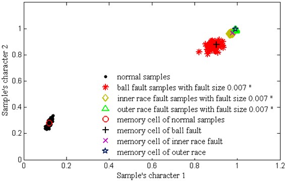
Table 5Used parameters in V-AIR for bearing data

Used parameters	The parameter value
Mutation rate	0.6
Average stimulation threshold	0.9
Clonal rate	50
Number of resources allowed in V-AIR	40
$k$ value for $k$ -weight nearest neighbor	1
$r$ value	0.4
$δ$ value	0.0075
$E_{t}$ value	0.001

5.2. The fault diagnosis of reciprocating compressor valves

The reciprocating compressor is a class of large general machinery widely used in petroleum chemical industry, mining, refrigeration and other industries. Its structure is complex, widely excitation source and the vibration is mainly put on multi-source impact signal such as air flow in and out of the cylinder, valve plates dropped into the seat or piston striking the block etc., which can’t be diagnosed by the traditional fault diagnosis methods.

To large reciprocating compressor, valve is the key components and according to some statistics, more than 60 % of the failure happens on valve. As valve is a typical reciprocating working part, it needs to be monitored and diagnosed based on intelligent fault diagnosis techniques.

Fig. 9 and Fig. 10 show the test site condition and vibration testing principle respectively. In the valve vibration monitoring, we used the high-frequency acceleration sensor with measurement frequency range 0.0002-10 kHz to gather the high frequency vibration signal of valve. The collected signal is transmitted to computer through 32 channel programmed multifunctional signal conditioner and intelligent data collection analyzer, which prepares for the subsequent data analysis. The sample length is 200000 points with sampling frequency 50 kHz and 200 groups of data samples for each fault condition.

Fig. 9The test site condition

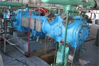
a) The tested reciprocating compressor

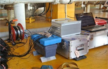
b) The used test instruments

Fig. 10The reciprocating compressor structure and the vibration testing principle

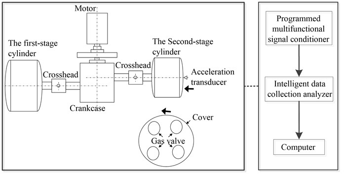
Fig. 11 gives the vibration signal of valve gap, plate fracture and spring deficiency fault. Due to the shock wave and impact time changing all the time, it is very difficult to detect the symptom of time domain waveform. Thus, in order to effectively diagnose the reciprocating compressor valve failure, we use the method of V-AIR for fault identification. Fig. 12 shows the distribution of training samples and $V$ - $m c_{h} s$ with different failure state, which is also disposed by PCA. In the V-AIR method, 100 groups of data samples are used for training with the rest 100 groups of data samples for testing. From Fig. 12, we can learn that different fault samples are completely non-linear separable and have different concentration degree.

Fig. 11The time domain vibration waveform of reciprocating compressor valve

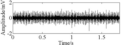
a) The normal vibration signals

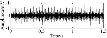
b) The spring deficiency fault vibration signals

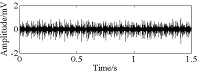
c) The valve gap fault vibration signals

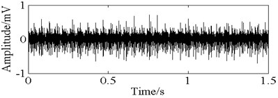
d) The plate fracture fault vibration signals

Like the method used in bearing analog fault diagnosis, Tables 6 and Table 7 show the average classification accuracy of 10 times test and the parameter values used in V-AIR respectively. It can be seen that the proposed V-AIR algorithm can effectively classify all kind of fault samples in the highly nonlinear separable condition: the testing accuracy for the normal samples are 89.5 % with 86 number of memory cells; with only 1 memory cell, the plate fracture and spring deficiency fault reach 90.5 % and 90.4 % respectively; for the value gap fault, it is 95.2 %. Thus, the result proves that V-AIR is a useful method in equipment fault diagnosis.

Fig. 12The training samples of reciprocating compressor valve fault and their memory cells

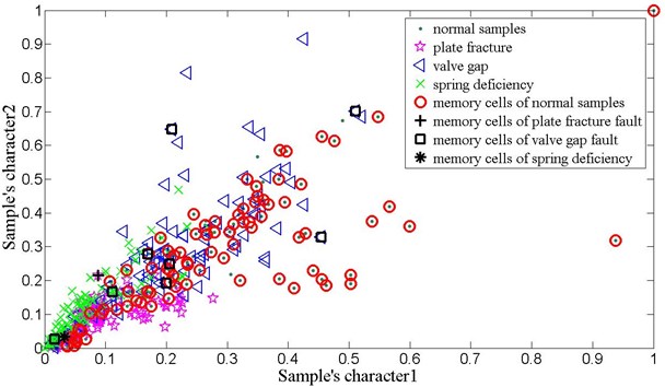
Table 6The reciprocating compressor valve fault classification accuracy of V-AIR

Type of samples	Number of memory cells	The classification accuracy of V-AIR (%)
Type of samples	Number of memory cells	Accuracy	Standard deviation
Normal samples	86	89.5	0.5
Plate fracture fault	1	90.5	0.3
Value gap fault	9	95.2	0.2
Spring deficiency fault	1	90.4	0.6

Table 7Used parameters in V-AIR for reciprocating compressor valve fault

Used parameters	The parameter value
Mutation rate	0.6
Average stimulation threshold	0.5
Clonal rate	100
Number of resources allowed in V-AIR	40
$k$ value for $k$ -weight nearest neighbor	1
$r$ value	0.75
$δ$ value	0.02
$E_{t}$ value	0.001

6. Conclusions

In this study, the inhibition mechanism between antibodies of AIRS that is among the most important classification systems of Artificial Immune Systems was changed with a new one that was formed with combining mutation. The fixed weight memory cells were also replaced by the variable weight memory cells with the weight changing according to the training samples’ density distribution. After training, the $k$ -weight nearest neighbor algorithm is used to determine the classes of test samples.

In the application phase of this study, four important UCI datasets: Diabetes, Ionosphere, Sonar and Iris were used. In the data classifications stage, the analyses were conducted both for the comparison of reached classification accuracy with other classifiers in UCI web site and the effects of the number of memory cells. According to the application results, V-AIR showed a considerably high performance with regard to the classification accuracy for all of the four dataset. The reached classification accuracy of V-AIR for the Diabetes, Ionosphere, Sonar and Iris were 74.5 %, 96.3 %, 86.8 % and 97.3 % respectively, which were all higher than the AIRS method. V-AIR is going one step ahead than the original AIRS with the aid of improvements done in the algorithm. The proposed change in this study has not only produced very satisfactory results, but also decreased the number of memory cells for some UCI datasets.

As an application example, the V-AIR also shows high classification accuracy for bearing data with only one memory cell for a kind of bearing data. In the process of reciprocating compressor valve fault diagnosis, it also shows great fault diagnosis effect. Thus, this method can be used for fault diagnosis successfully.

References

Dasgupta D., Yu S., Nino F. Recent advances in artificial immune systems: models and applications. Applied Soft Computing, Vol. 11, Issue 2, 2011, p. 1574-1587.

Search CrossRef
Dasgupta D., Yu S., Majumdar N. S. MILA-multilevel immune learning algorithm and its application to anomaly detection. Soft Computing, Vol. 9, Issue 3, 2011, p. 172-184.

Search CrossRef
Forrest S., Perelson A. S., Allen L., et al. Self-nonself discrimination in a computer. IEEE Computer Society Symposium on Research in Security and Privacy, 1994, p. 202-212.

Search CrossRef
Mousavi M., Abu Bakar A., Zainudin S., et al. Negative selection algorithm for dengue outbreak detection. Turkish Journal of Electrical Engineering and Computer Sciences, Vol. 21, Issue 2, 2013, p. 2345-2356.

Search CrossRef
Gonzalez F., Dasgupta D., Kozma R. Combining negative selection and classification techniques for anomaly detection. Congress on Evolutionary Computation, 2002, p. 705-710.

Search CrossRef
González F., Dasgupta D., Gómez J. The effect of binary matching rules in negative selection. Genetic and Evolutionary Computation – GECCO, First Edition, Springer Inc., Chicago, 2003.

Search CrossRef
Ji Z., Dasgupta D. V-detector: an efficient negative selection algorithm with “probably adequate” detector coverage. Information Science, Vol. 179, Issue 10, 2009, p. 1390-1406.

Search CrossRef
Ji Z., Dasgupta D. Real-valued negative selection algorithm with variable-sized detectors. Genetic and Evolutionary Computation – GECCO, First Edition, Springer Inc., Seattle, 2004.

Search CrossRef
Shapiro J. M., Lamont G. B., Peterson G. L. An evolutionary algorithm to generate hyper-ellipsoid detectors for negative selection. Conference on Genetic and evolutionary computation, First Edition, ACM., Washington, 2005.

Search CrossRef
Zeng J., Tang W., Liu C., et al. Real-valued negative selection algorithm with variable-sized self radius. Information Computing and Applications, First Edition, Springer Inc., Chengdu, 2012.

Search CrossRef
Jerne N. K. Towards the network theory of the immune system. Annales d’Immunologie, Vol. 125, 1974, p. 373-389.

Search CrossRef
Farmer J. D., Packard N. H., Perelson A. S. The immune system adaptation and machine learning. Physica D, Vol. 22, 1986, p. 187-204.

Search CrossRef
Ultsch A. U*-Matrix: a Tool to Visualize Clusters in High Dimensional Data. Technical Report, Philipps-University Marburg, Marburg, Germany, 2003.

Search CrossRef
Kohonen T. Self-organizing Maps. Springer Inc., Berlin, 2001.

Search CrossRef
Bezerra G. B., Barra T. V., De Castro L. N., et al. Adaptive radius immune algorithm for data clustering. 4th International Conference on Artificial Immune Systems, First Edition, Springer Inc., Banff, 2005.

Search CrossRef
Timmis J., Neal M., Hunt J. An artificial immune system for data analysis. Biosystems, Vol. 55, Issues 1-3, 2000, p. 143-150.

Search CrossRef
Timmis J., Neal M. A resource limited artificial immune system for data analysis. Knowledge Based System, Vol. 14, Issue 3-4, 2001, p. 121-130.

Search CrossRef
Watkins A. B. AIRS: a Resource Limited Artificial Immune Classifier. Mississippi State University, Mississippi, 2001.

Search CrossRef
Polat K., Şahan S., Güneş S. A new method to medical diagnosis: Artificial immune recognition system (AIRS) with fuzzy weighted pre-processing and application to ECG arrhythmia. Expert System Application, Vol. 31, Issue 2, 2006, p. 264-269.

Search CrossRef
Polat K., Güneş S., Tosun S. Diagnosis of heart disease using artificial immune recognition system and fuzzy weighted pre-processing. Pattern Recognition, Vol. 39, Issue 11, 2006, p. 2186-2193.

Search CrossRef
Polat K., Şahan S., Kodaz H., et al. Breast cancer and liver disorders classification using artificial immune recognition system (AIRS) with performance evaluation by fuzzy resource allocation mechanism. Expert System with Application, Vol. 32, Issue 1, 2007, p. 172-183.

Search CrossRef
Ozsen S., Gunes S. Performance evolution of a newly developed general-use hybrid AIS-ANN system: AaA-response. Turkish Journal of Electrical Engineering and Computer Sciences, Vol. 21, Issue 6, 2013, p. 1703-1709.

Search CrossRef
Li D. Y., Du Y. Artificial Intelligence with Uncertainty. First Edition, National Defense Industry Press, Beijing, 2005.

Search CrossRef
Wang S. L., Cheng G. Q., Li D. Y., et al. A try for handling uncertainties in spatial data mining. 8th International Conference on Knowledge-Based Intelligent Information and Engineering Systems, First Edition, Springer Inc., Wellington, 2004, p. 149-153.

Search CrossRef
Igawa K., Ohashi H., et al. A negative selection algorithm for classification and reduce of the noise effect. Applied Soft Computing, Vol. 9, Issue 1, 2009, p. 431-438.

Search CrossRef
Zheng H. B., Chen X. Z., Li Z. Y., et al. Implementation and application of a neural network fault diagnosis system based on wavelet transform. Transactions of the Chinese Society of Agricultural Machinery, Vol. 5, Issue 1, 2002, p. 73-76.

Search CrossRef

About this article

Received

04 December 2014

Accepted

05 May 2015

Published

15 August 2015

SUBJECTS

Fault diagnosis based on vibration signal analysis

Keywords

V-AIR

data potential field

weight optimizing

network inhibition

combining mutation

Acknowledgements

This work was supported by National Natural Science Foundation of China (50475183), the Specialized Research Fund for the Doctoral Program of Higher Education (20103 108110006) and Shanghai Science and Technology Commission Basic Research Project (11JC140 4100).

This is an open access article distributed under the Creative Commons Attribution License, which permits unrestricted use, distribution, and reproduction in any medium, provided the original work is properly cited.