Intelligent modelling and active vibration control of flexible manipulator system

1. Introduction

Manipulators are one of the important appendages of most of dynamic systems. Owing to some functional applications they have been extensively utilized in aero investigations [1], biomedical applications [2], robotic system [3] and many other fields that require heavy, tedious and accurate structural minipulations. In most cases where the need for less energy consumption, increase of operation speed and optimization of dimensions, the flexible manipulator is the preferable choice over its rigid counterpart.

Apart from useful contribution of flexible manipulator, its low stiffness characteristic evolves drawbacks of unwanted vibration or chaotic motion especially when it is stimulated by any external loads or maneuvered by simple torque at some points. This extra oscillation causes time delay and also wastes a great deal of energy. Quite recently, considerable attention has been paid to deal with flexible manipulator weaknesses. A solution would be designing a proper control system in order to suppress the unwanted oscillation. The controller can be selected in active or passive configuration. In system control strategy, if the accurate modelling of flexible manipulator is implemented in the primitive stage, the system will yield satisfactory response. Recently, research on modelling and control of flexible manipulator has become very popular with a variety of approaches. Tang et al. [4] presented the modelling of single flexible manipulator by using Lagrange formulation, where the trajectory and vibration control based on approximation of neural network (NN) and the concept of sliding mode control (SMC) are considered. Feliu et al. [5] proposed lumped masses to model the single flexible manipulator and feedforward controller is designed as control scheme. In [6] the assumed mode method (AMM) was used to obtain the mathematical model of two flexible links, while the neural adaptive control was adapted for control strategy. However, dealing with huge differential equations for modelling of flexible manipulater by classical approach is cumbersome, so the system identification method utilizes the differences equations to model the dynamic system [7]. In a recent paper by Duarte et al. [8] the black box technique is applied to present the dynamic model of flexible link and vibration cancelation is done by using the H_∞ control scheme. Franke et al. [9] developed the frequency response function (FRF) to extract the transfer function of flexible manipulator, and for eliminating the vibration feedforward input the shaping was carried out using strain feedback control. The most interesting approach to this issue has been proposed by [10] in which the soft computing method is implemented for trajectory and vibration control. Also, beam structural analysis could be considered as an insight of modelling and control for flexible manipulator [11].

In this paper the author offers another alternative system identification technique in which autoregressive with exogenous input (ARX) model as linear structure and NARX model as nonlinear structure are signified. In short, the ARX model is one where its parameters are estimated by conventional recursive least square (RLS) approach. For NARX model the nonparametric model estimation is done by artificial neural network algorithm. Finally the proportional integral derivative (PID) controller is utilized for both models for eliminating the undesirable vibration. The performance of PID controller is also evaluated by applying different disturbances on the control system.

2. The flexible manipulator system

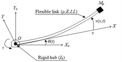
Fig. 1 depicts a typical single-link flexible manipulator. The single-link flexible manipulator is considered a pinned-free arm with length $L$ and tip mass $M_p$, attached to either a rigid or flexible hub. Here, the rigid joint is considered with arm inertia $I_t$. As in most cases an input torque $\tau \left(t\right)$ is applied at the hub by an electrical motor. $E$, $I$ and $\rho$ represent the Young modulus, second moment of inertia and mass density per unit length, respectively, of the arm. In this study, the motion of the flexible manipulator is defined in the $X_{0}O{Y}_0$ and $XOY$ axis systems, as stationary and moving coordinates, respectively. The overall displacement $w(x,t)$ is consisted of angular displacement $\theta \left(t\right)$ and elastic deflection $\vartheta (t,x)$ which can be described as:

Fig. 1Typical flexible manipulator arm

The governing equation of the flexible manipulator, by considering the boundary and initial conditions, is obtained as:

The analytical method can be used to deal with the fourth order PDE. Most studies do not take into account the solution of Eq. (2) by analytical method directly, because by changing the boundary conditions and adding more than one flexible link, solving of such PDEs becomes thorough. So, other alternative methods have been used to present the dynamic model of flexible manipulator with different number of links. For instance, by truncating the continuous link into finite number of subsystems or elements and applying the assume mode method (AMM) [12] and finite element method (FEM) [13] a discrete model could be presented. The dynamic motion of the flexible manipulator can be extracted by incorporating the energy principle in the Lagrange or Hamilton formulations. The lumped parameters system is also used [5] to derive the dynamic equation of single link flexible manipulator, but with less accuracy than FEM and AMM. In the present study, to derive the mathematical model of the flexible manipulator system, the system identification technique is applied, as a novel approach, for modelling of dynamic systems possessing complicated dynamic characteristics and encountering with some uncertainties such as nonlinear behavior, changeable mass, stiffness and damping.

3. System identification

Identification of dynamic systems which have flexibility has attracted researchers recently. In this work, linear system identification is carried out by using the ARX model and nonlinear system identification is conducted using NARX model. In addition to choosing the model structure, the input and output signals, as discrete set of data, must be assigned as well. Input and output data can be obtained from experimental test of real system. The system is excited with test signal and its response measured. When the experiment test is not available other alternative method can be carried out to simulate the system. In this study, the input and output signal detection is done by finite difference (FD) method that is described in [14].

3.1. Linear system identification

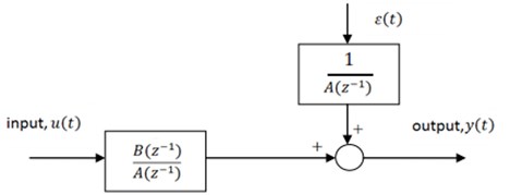
A linear model using autoregressive with exogenous input (ARX) model is presented in this study. Fig. 2 illustrates the schematic of the ARX model. Using the symbols in Fig. 2 the model function can be written as:

3

$y\left(t\right)=\frac{B\left(z^{-1}\right)}{A\left(z^{-1}\right)}u\left(t\right)+\frac{1}{A\left(z^{-1}\right)}\epsilon \left(t\right),$

where, $A\left(z^{-1}\right)$ and $B\left(z^{-1}\right)$ are polynomials and $u\left(t\right)$ is the input data and $y\left(t\right)$ is the output data while $ϵ\left(t\right)$ is the white noise. By neglecting the noise effect and rewriting Eq. (3) we have:

4

$y\left(t\right)A\left(z^{-1}\right)=B\left(z^{-1}\right)u\left(t\right),$

where:

5

$A\left(z^{-1}\right)=1+a_1{z}^{-1}+a_2{z}^{-2}+\dots +a_n{z}^{-n},$

6

$B\left(z^{-1}\right)=b_0+b_1{z}^{-1}+b_2{z}^{-2}+\dots +b_m{z}^{-m}.$

By substituting Eqs. (5) and (6) into Eq. (4) the model in Eq. (3) can be shown as:

7

$y\left(t\right)=-\sum _{i=0}^n{a}_1{z}^{-1}+a_2{z}^{-2}+\dots +a_n{z}^{-n}+\sum _{i=0}^n{b}_1{z}^{-1}+b_2{z}^{-2}+\dots +b_m{z}^{-m},$

or:

8

$y\left(t\right)=-\sum _{i=0}^n{a}_i{z}^{-i}+\sum _{i=0}^m{b}_i{z}^{-i},a_0=1,b_0=0.$

In both discrete polynomials, $n$ and $m$ refer to the order of the function where $n\ge m$. $z^{-n}$ and $z^{-m}$ are backshift operators and $y\left(t\right)$ is the sampled output.

Fig. 2ARX model structure

3.1.1. Parameters estimation

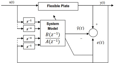
By signifying the ARX model, we can estimate the model parameters $[a_1,\dots ,a_n,b_1,\dots ,b_m]$ by applying the recursive least square method (RLS). Fig. 3 shows the schematic of RLS method. By rewritting Eq. (7) in the standard form the mathematical definition of RLS is presented as:

9

$y\left(t\right)=\phi \left(t\right)\beta ,$

where $y\left(t\right)$ is the actual output, $\phi \left(t\right)$ is the regressor that includes the input and output data and $\mathrm{\beta }\mathrm{}$are the system parameters. Consequently, Eq. (9) can be presented in the matrix form of Eq. (10) by replacing $z^{-n}$ with $y\left(t-n\right)$ and $z^{-m}$ with$y\left(t-m\right)$:

10

$y\left(t\right)=\left[\begin{array}{ccc}-y(t-1)& \cdots & -y(t-n)\end{array}\begin{array}{ccc}u(t-1)& \cdots & u(t-m)\end{array}\right]\left[\begin{array}{c}{a}_1\\ \begin{array}{c}⋮\\ a_n\\ \begin{array}{c}{b}_1\\ ⋮\end{array}\end{array}\\ b_m\end{array}\right].$

By employing the cost function and adding new parameters the unknown parameters in Eq. (9) can be estimated by Eq. (11):

11

$\widehat{\beta }\left(t+1\right)=\widehat{\beta }\left(t\right)+p\left(t+1\right)\phi \left(t+1\right)ϵ\left(t+1\right).$

Two new parameters are introduced, namely $p\left(t+1\right)$ as arbitrary value and $ϵ\left(t+1\right)$ as error variable, and they can be defined as:

12

$p\left(t+1\right)=p\left(t\right)\left[I-\frac{\phi \left(t+1\right){\phi }^T\left(t+1\right)p\left(t\right)}{\gamma +{\phi }^T\left(t+1\right)p\left(t\right)\phi \left(t+1\right)}\right],$

13

$ϵ\left(t+1\right)=y\left(t+1\right)-{\phi }^T\left(t+1\right)\widehat{\beta }\left(t\right).$

Note that in Eq. (12), $\gamma$ is the forgetting factor that varies from 0 to 1. Finally, the estimated output $\widehat{y}\left(t\right)$ in Eq. (14) is obtained by replacing the estimated parameter $\beta$ by $\widehat{\beta }$ in Eq. (9):

14

$\widehat{y}\left(t\right)=\phi \left(t\right)\widehat{\beta }.$

However, the proposed model using the estimated parameter is optimum when the mean-square error (MSE) gets minimized:

15

$\mathrm{M}\mathrm{S}\mathrm{E}=\frac{1}{N}\sum _{i=1}^N{\left(\left|y\left(i\right)-\widehat{y}\left(i\right)\right|\right)}^2.$

In Eq. (15), $y\left(i\right)$ and $\widehat{y}\left(i\right)$ are the actual and estimated output respectively, and $N$ denotes the number of sampled data.

Fig. 3Diagram of RLS algorithm

3.1.2. RLS result

By considering the finite difference method, Fig. 4 and 5 show the results [14] of the input signal (as bang-bang torque $\tau \left(t\right)$ imposed at link hub) and response output signal (manifested as tip displacement). These two signals are sampled with period of 0.04 ms into 68842 points and normalized between –1 and 1.

Fig. 4Sampled input signal, bang-bang torque

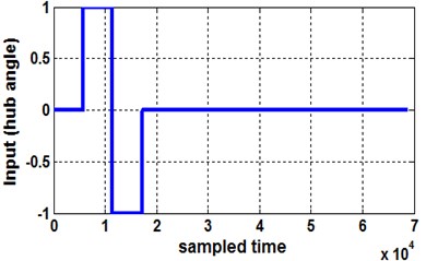
Fig. 5Sampled output signal, tip displacement

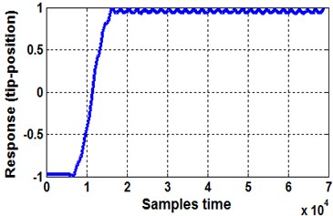
Consider the implementation of the two described signals into the ARX model. The modelling becomes more reliable when the estimation process is divided into training and testing steps. In this case the model parameters are estimated by using half of the data and tested by employing the entire data in order to achieve the adaptive model with the minimum mean square error (MSE). After conducting the system identification process, the model order of 2 is found to be the best model with minimum MSE of 2.8546×10^-8.

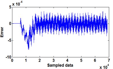
The parameters of the second order model, namely $[a_1,a_2,b_1,b_2]$ in Eqs. (5) and (6), are extracted by making the regressor matrix $\phi \left(t\right)$in Eq. (10) create $p\left(t+1\right)$ and $ϵ\left(t+1\right)$in Eqs. (12) and (13) respectively. Then the desired parameters $\widehat{\beta }\left(t\right)$ would be estimated by Eq. (11) in vector form, where$a_0=\text{1,}$$a_1=\text{–0.5,}$$a_2=\text{–0.5,}$$b_0=\text{0,}$$b_1=$–2.0733×10^-6, $b_2=$ –2.091×10^-6. On the other hand, the estimated output is evaluated by Eq. (14) which tries to minimize the MSE as well. The above formulation are programmed using Matlab software. Finally, by inserting the adapted parameters in Eq. (3) the transfer function of ARX model can be found, as presented by Eq. (16). The actual and estimated responses, with their errors, are illustrated in Figs. 6 and 7 graphically:

16

$G\left(z\right)=\frac{y\left(z\right)}{u\left(z\right)}=\frac{-2.0733\times {10}^{-6}{z}^{-1}-{2.091\times 10}^{-6}{z}^{-2}}{1-0.5z^{-1}-0.5z^{-2}}.$

Fig. 6Actual and estimated output

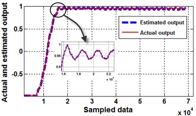
Fig. 7Error between actual and estimated output

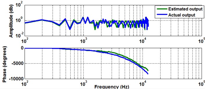
For validation of the linear ARX model the frequency response function (FRF) for both actual and estimated output are illustrated in Fig. 8. As it is shown in the frequency domain the estimated output follows the same trend as actual output. All frequencies are captured using the proposed linear model but with negligible phase differences in high frequency domain. It is noted that the active vibration control for flexible manipulator system is intended to work in low frequency range.

Fig. 8Frequency response function for actual and estimated output

3.2. Nonlinear system identification

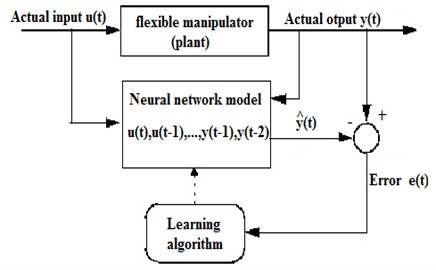
In this section nonlinear system identification is discussed in relation to nonlinear autoregressive with external (exogenous) input (NARX) model. Fig. 9 shows the nonlinear estimation process using the artificial neural network (NN) algorithm for NARX model in the iterative process. As rule of thumb the NN uses the past input and output data to estimate the present output as delayed input and output variables (regressors) namely, $y\left(t-1\right)$, $y\left(t-2\right)$,…, $y\left(t-na\right)$, $u\left(t\right)$, $u\left(t-1\right)$,…, $u(t-nb-1)$. In this study the NN is trained by using the Levenberg-Marquardt back propagation in order to achieve the minimum error. Nonlinear identification process has the same scenario with the formerly described linear identification, which means making the nonlinear structure using the half of the data and testing the extracted model using the entire data to obtain the adaptive model with minimum MSE. In this work all numerical calculations were computed using the software tool from Mathworks Inc. which include MATLAB, Simulink and control environments. In the literature this type of system identification is known as black box technique because the model function is not physically significant.

Fig. 9Schematic of NARX NN structure

3.2.1. Neural network result

By altering the configuration of neural network (NN) algorithm such as different time delay and number of neurons in the hidden layer the best model with minimum MSE can be accurately achieved. In this case only one hidden layer is selected and the best model is obtained by choosing 8 neurons and a time delay of 6, thus obtaining an MSE of 8.770×10^-12 in the training process, see Table 1. Finally the black box model is implemented for estimating output from the entire data testing process. This model is depicted in Fig. 10 with MSE 3.4×10^-5 for entire data. The estimated output and actual output with their absolute error are illustrated in the Figs. 11 and 12 respectively.

Fig. 10NARX NN model simulation

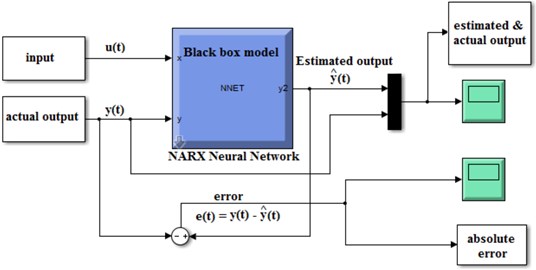
Fig. 11Actual and estimated output

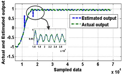
Fig. 12Error between actual and estimated output

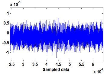
Table 1Values of MSE in neural network configuration

Number of neurons	Delay = 2 MSE	Delay = 4 MSE	Delay = 6 MSE	Delay = 8 MSE	Delay = 10 MSE
2	2.0486×10-8	1.0249×10-9	9.867×10-9	8.554×10-11	4.14×10-9
4	1.15×10-8	2.189×10-7	3.215×10-7	1.132×10-9	1.22×10-5
6	2.023×10-11	1.17×10-9	8.296×10-6	5.426×10-9	6.76×10-8
8	2.058×10-11	1.37×10-7	8.770×10-12	6.24×10-9	1.036×10-5
10	2.055×10-11	4.75×10-6	2.667×10-11	9.33×10-7	2.23×10-6

Fig. 13Validation results

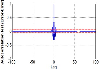
a) Auto-correlation ${\varnothing }_{ee}\left(\tau \right)$

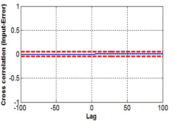
b) Cross-correlation ${\varnothing }_{ue}\left(\tau \right)$

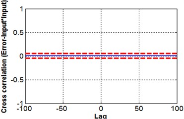
c) Cross-correlation${\varnothing }_{u^{2}e}\left(\tau \right)$

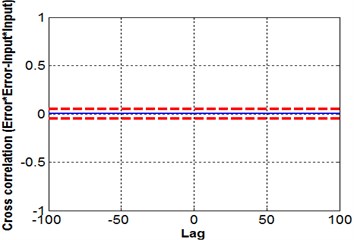
d) Cross-correlation ${\varnothing }_{u^2{e}^2}\left(\tau \right)$

e) Cross-correlation ${\varnothing }_{e\left(eu\right)}\left(\tau \right)$

3.2.2. Model validation

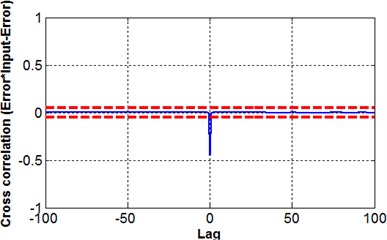
Previously, the system identification technique was implemented by dividing input-output data into two sets of data for training and for testing process to show the model adaptiveness to a new set of data. For linear model the FRF was utilized to validate the model. However, predictive capability of proposed nonlinear model by system identification technique should be validated by some statistical method such as the correlation test [15], as given in Eq. (17). A model is validated when these equations are satisfied, in other words, when the residuals (errors) are uncorrelated with linear and nonlinear combinations of past input and output:

17

${\varnothing }_{e\left(eu\right)}\left(\tau \right)=E\left[e\left(t\right)e\left(t-1-\tau \right)u\left(t-\tau \right)\right]=0,\tau \ge 0,$
${\mathrm{\varnothing }}_{u^2{e}^2\mathrm{}}\left(\tau \right)=E\left[u^2\left(t-\tau \right)-u^2\left(t\right)e^2\left(t\right)\right]=0,\mathrm{}\mathrm{}\mathrm{}\forall \tau ,$
${\mathrm{\varnothing }}_{ue}\left(\tau \right)=E\left[u\left(t-\tau \right)e\left(t\right)\right]=0,\mathrm{}\mathrm{}\mathrm{}\forall \tau ,$
${\varnothing }_{u^{2}e}\left(\tau \right)=E\left[u^2\left(t-\tau \right)-u^2\left(t\right)e\left(t\right)\right]=0,\forall \tau ,$
${\varnothing }_{ee}\left(\tau \right)=E\left[e\left(t-\tau \right)e\left(t\right)\right]=\delta \left(\tau \right),$

where $u\left(t\right)$ is input, $e\left(t\right)$ is the predicted error, ${\mathrm{\varnothing }}_{ue}\left(\tau \right)$ indicates the cross-correlation function between $u\left(t\right)$ and $e\left(t\right)$ and $\delta \left(\tau \right)$ is an impulse function. For nonlinear system identification all five equations should be used [14]; in the present case a 95 % confidence band indicates that the proposed NN model satisfies all five equations, see Fig. 13.

4. Feedback controller

In order to eliminate the tip vibration of flexible link manipulator active vibration PID control scheme is conducted for both ARX and NARX models in the feedback control strategy. In this study discrete modelling for the sampled time is proposed, and the digital PID controller is selected for both linear and nonlinear models. The PID controller parameters are automatically tuned by using the interactive design mode technique.

Fig. 14System response with controller

4.1. Active vibration control for linear model

In this section the ARX model is embedded into the feedback control loop, see Fig. 15. The adaptive and robust capability of PID controller can be evaluated by altering the disturbance signal. The parameters of the designed PID controller in presence of a first disturbance, a step signal, is stored when different disturbance signal is imposed to the system. In this case the repeating sequence signal is utilized as another alternative disturbances signal. The response of system to a step input reference signal, with two different disturbance is depicted in Fig. 14. As expected the system vibration is canceled and stabilized by PID controller with 6 % overshoot and 0.002 steady state error.

Fig. 15Digital PID controller with discrete system in the feedback loop

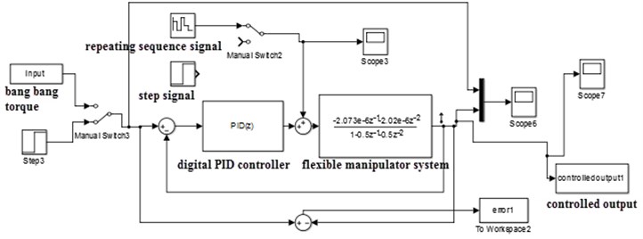
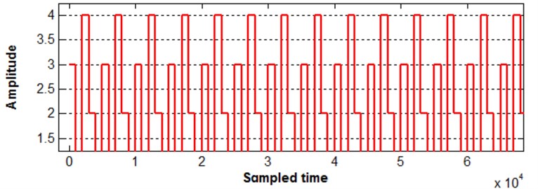
To evaluate how well the system performs in the feedback control loop, the bang-bang torque is imposed as a reference signal. From Fig. 16, with the new reference signal the controller stabilizes system and damps the extra vibration as well. The disturbance signal profile is illustrated in Fig. 17 as a repeating sequence signal.

Fig. 16System response to the bang-bang torque as reference signal

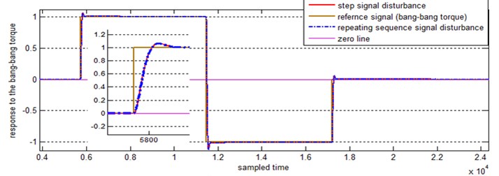
Fig. 17Repeating sequence disturbance signal

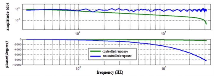
By applying the frequency response function (FRF) for both controlled and uncontrolled systems that are stimulated by bang-bang torque, the performance of the PID controller can be evaluated from the well-damped amplitudes of response in the FRF result, shown in Fig. 18.

Fig. 18Frequency response of the bang-bang torque for controlled and uncontrolled system

4.2. Active vibration control for nonlinear model

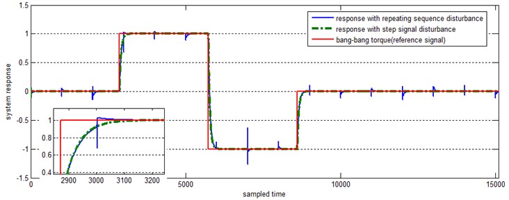
In this section the proposed NARX neural network model is utilized in the feedback scheme with digital PID controller. The control system is depicted in Fig. 19 and the response of the system to a reference signal (step signal) in the presence of two different disturbances namely, step signal and repeating sequence signal, is illustrated in Fig. 20. In order to follow the same scenario with presented control scheme for linear system in the previous section, the bang-bang reference torque signal is exerted into the control system to evaluate the control capability with respect to different reference signals and disturbances.

Fig. 19Digital PID controller with black box system in the feedback loop

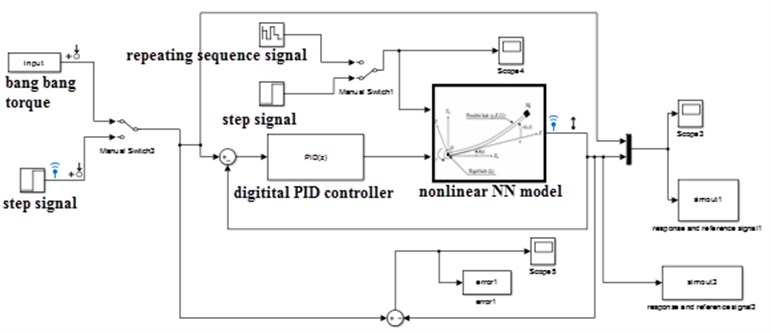
Fig. 20System response to the step signal with two different disturbances

As illustrated in Fig. 21, the PID controller in the presence of bang-bang torque shows a desirable response (without overshooting). The step signal is imposed as disturbances, by applying a new disturbance, such as repeating sequence signal. Some peaks are seen in the controlled response.

Fig. 21System response to the bang-bang torque as reference signal

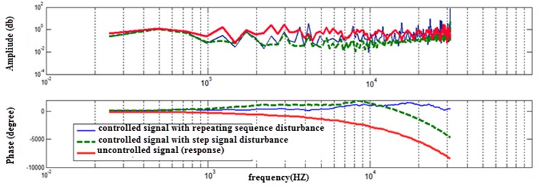
The FRF is taken into account for evaluating the robustness of PID controller on nonlinear NARX neural network model in the case of a step signal disturbance. From Fig. 22 it can be seen that the PID controller completely attenuates the vibration of the flexible manipulator by reducing the amplitude for the entire frequency domain. It is also observed that the amplitude is augmented when imposed by a repeating sequence disturbance in the high frequency region. However, the flexible manipulator system is concerned with active vibration control in the low frequency domain rather than high frequency domain.

Fig. 22Frequency response to the bang-bang torque for controlled and uncontrolled system

5. Conclusions

This study has demonstrated a PID controller design for linear and nonlinear modeling of flexible manipulator with the aim of suppressing unwanted vibration due to external excitations. A significant implication is that the linear model (ARX) shows a better estimation with MSE of 2.8546×10^-8 compared to nonlinear model (NARX) with MSE of 3.4×10^-5. The excellent supression in the linear model can be verified from test data acquisition using finite difference method, because the FD method estimates a linear model for nonlinear system. In addition, proposed models are validated by employing FRF and correlation test for linear and nonlinear model respectively. The PID controller was implemented in both models to cancel the vibration. In the presence of input signal and disturbances in the control loop, the amplitude of the system response for entire frequency domain is canceled for the linear model. However, the amplitude of the system response for nonlinear model is barely attenuated especially in the low frequency region. The most likely explanation of the different PID controller performance in both models is that the parametric PID controller is well adapted with parametric linear model rather than nonlinear and nonparametric models. The next stage of this research is experimental confirmation of our simulation and also designing the nonlinear control scheme for the proposed NARX model.