Abstract
As one of the most important aspects of PHM in many application domains, health monitoring and management could maximize the equipment effectiveness within the allowed health ranges. This paper proposes a novel approach to assess the equipment health based on hidden semi-Markov model (HSMM), which is an extension of HMM and does not follow the unrealistic Markov chain assumption to provide more powerful modeling and analysis capability for real problems. With training the standard health state HSMM model by normal state data, the test data is inputted into the trained model in order to calculate the corresponding relative divergence, which is the deviation extent from the standard health state model. Then we can obtain the health index model for the equipment health monitoring and measurement. Moreover, the proposed HSMM based method is applied to the draught fan and showed to be effective.
1. Introduction
With technological development brought in increased performance, function and complexity of the equipment system to achieve automation, the Condition Monitoring [1] and Fault Diagnosis [2] is generated.
However, the equipment state is often difficult to observe directly and the actual equipment health state can only be expressed or reasoned out from the output symptoms. Thus an appropriate method called Hidden Markov Model (HMM) has attracted increasing attentions in the equipment diagnostics and prognostics fields. However, these HMM based methods are limited to some unrealistic assumptions, so the new HSMM methods are derived that does not follow the Markov chain assumption. Otherwise, the traditional health assessment based on HMM/HSMM usually need various machine operating data for different training HMM or HSMM models. However, the required data can barely get in most situations. Therefore, we proposed an HSMM based method for equipment health assessment, which only required the health/normal state data for training. By calculating the corresponding relative divergence from the standard health state to the test states, we can obtain the equipment health index. Furthermore, the proposed approach is applied to the draught fan and showed to be effective.
1.1. Hidden semi-Markov model (HSMM)
The Hidden Markov Model (HMM) is a probability model for describing the statistical properties of stochastic process [3]. In parallel with the extensive use of HMMs in applications [4] and with the related statistical inference work, a new type of model was derived, initially in the domain of speech recognition. A recent book that covers much work on the field is Barbu V. S. et al. (2008) [5]. Because the main drawback of hidden Markov models requires that the sojourn time in a state be geometrically or exponentially distributed, so Ferguson (1980) proposed a model called a hidden semi-Markov model that allows arbitrary sojourn time distributions for the hidden process.
Since then HSMM has been applied in many scientific and engineering areas, such as speech/handwriting recognition, gene identification, human activity prediction and network anomaly detection [6, 7]. An important example of practical interest of hidden semi-Markov models is GENSCAN [8], a program for gene identification which developed by Chris Burge at Stanford University. Although HMM and HSMM have been well studied and applied, there are few papers of HSMM in the state recognition and fault diagnosis fields, mainly represented by Shun Zheng Y., Dong Ming and David He. Shun Zheng Y. also pointed a new and computationally efficient forward–backward algorithm for HSMM with missing observations and multiple observation sequences. And an integrated platform based on HSMM for multi-sensor equipment diagnosis and life prognosis is presented [9]. Then Dong Ming [10, 11] proposed a segmental HSMMs based method for performing both diagnosis and prognosis in a unified framework. Furthermore, Peng Ying in his paper proposed three types of aging factors that discount the probabilities of staying at current state while increasing the probabilities of transitions to less healthy states [12]. An R package for analyzing hidden semi-Markov models can also be found in Bulla et al. [13].
2. Hidden semi-Markov model based equipment health assessment framework
2.1. Parameters of hidden semi-Markov model
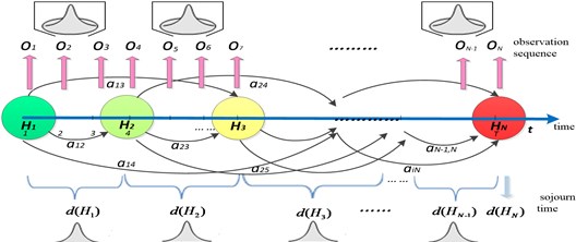
Suppose that the equipment health state has been classified into discrete hidden states and the equipment health degradation changes with time. Although the equipment health states are hidden, there is often some physical signal attached to the health states of the model as shown in Fig. 1. The complete specification of an HSMM consists of the following elements, described as.
The state transition probability distribution matrix is where , , , and is the number of health states and is the state at time in HSMM. The conditional probability distribution matrix of observing when given state is parameter represents the state duration distribution , , written as where state lasts time units. And the initial state probability distribution is , .
Fig. 1HSMM based health state transition

2.2. HSMM based three-step health assessment
The traditional health assessment based on HMM/HSMM all need different state data to get different training HMMs or HSMMs and input the test data to calculate the corresponding emission probabilities in these models. Then the hidden state is the one that generates the maximal emission probability. However, the required data is hard to capture and identify which state belonged in real applications. Therefore, we proposed an HSMM based method for equipment health assessment, which only required the health state data for training. This three-step health assessment based on HSMM includes training step, input step and deviation calculation step.
[Step 1] Learning/training step.
First all of the captured data should be analyzed for feature extraction, and a health standard HSMM is trained and the parameters are estimated by using only health/normal state training data set.
[Step 2] Input step.
On the basis of this trained health standard HSMM , we can obtain observation probability of the trained health model , where the other test data should be inputted to calculate the observation probabilities associate with the test states.
[Step 3] Deviation calculation step.
With calculating the corresponding relative Kullback-Leibler Divergence between the health/normal state and the unknown state, the health index can be obtained for equipment health assessment.
Define Kullback-Leibler Divergence (also known as Relative Entropy) as the variance between two probability distributions , [14]. With achieving the observation probability of the health state and the test state , the Kullback-Leibler Divergence represents the deviation extent from the standard health state can be calculated by Eq. (1):
The smaller the , the higher equipment health level is, and vice versa. When is greater than the threshold that depends on the performance requirements for equipment, the equipment has completely failed. Therefore, the equipment health index [0, 1] can be obtained through normalization.
3. Inference and leaning mechanisms for HSMM
3.1. Forward/backward algorithm
Baum proposed the Forward/backward algorithm for the emission probability , and the partial forward probabilities and partial backward probabilities are defined as follows.
1. The forward algorithm.
We define a forward variable described as the joint distribution of observation sequence and health state at time when given the model .
where the emission observation of state is and state is , represent the state lasts from to , and is the maximal duration time.
2. The backward algorithm.
Similar to forward variable, we define a backward variable as Eq. (3):
3.2. Baum-Welch based re-estimation algorithm
The training process is the adjusting and re-estimation the HSMM parameters in order to maximize the observation sequence probability when the parameters are unknown or inaccurate. There are many methods for learning such as Maximum Likelihood (ML), Maximum Mutual Information (MMI), Minimum Discriminate Information (MDI), and the most classical one is the Baum-Welch algorithm which is presented here.
In order to obtain the parameters of the hidden Markov model, note two variables first as following: We denote the posterior probability as , shown in Eq. (4):
Let Baum-Welch variable be , expressed as Eq. (5):
The parameters and usually have little effects on determining the initial values, but the initial , matrix are opposite and can be got by the K-means algorithm. Then the parameters can be obtained by Baum-Welch algorithm based re-estimation formulas as Eq. (6) until the observation probability converges to a pre-determined interval:
4. Case study
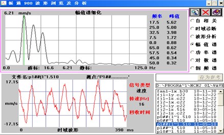
Take the rotational draught fan for case study in order to evaluate the equipment health by the proposed method. As the main factors influencing the draught fan include the bearing wear and dust accumulated on blade, we find that the bearing wear and loose gap of mating parts all lead to the additional vibration of fan body. So we could take the mechanical vibration signals which contain enough information for the fan’s health monitoring. Here the vibration data used for our test were captured by the accelerometer sensors on the fan body, and the wear test experiments data was collected from accelerometers by Two-Channel Data Collector#907 and Vibration Analyzer shown in Fig. 2.
Fig. 2Normal state amplitude spectrum analysis

We could obtain 3 sets of observation data respectively corresponding to the initial operating (normal) state, the bearing inner-race and out-race fault states, with 4 feature vector in each observation sequence, including the 1st, 2nd, 3rd and the 5th harmonics.
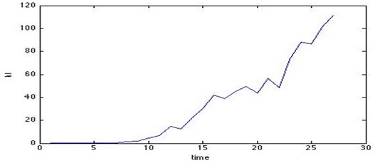
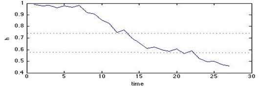
In fact, the majority of equipment performance or operation state would become degradation gradually and get into a worse state without maintenance. So the left-right HSMM without jumping was chosen. Denote the hidden states are 3, and the initial state is always health (normal). Here in the paper the initial state probability is [1, 0, 0]. After data preprocessing and feature extraction by principal component analysis, first the observation sequence of the normal state should be used by training the standard HSMM. According to the steps above, the standard HSMM parameters can be calculated until the observation probability converges. Generally, we take the for convenience. Then the Kullback-Leibler Divergence can be calculated by Eq. (1), shown in Fig. 3. And health index can be normalized, as shown in Fig. 4.
Fig. 3KL divergence curve with time

Fig. 4Health index curve with time

The result verifies that the changes of increasing Kullback-Leibler Divergence and the decreasing health index can sufficiently show the real state changes of the fan, and the trend of health index curve is quite same as the KL divergence curve. Therefore, the equipment real-time health can be easily mastered by assessing the health index and the maintenance decision can be conveniently made in time by monitoring the health index. Besides, this new HSMM based method also makes the relative distances to be more obvious even if data changes slightly.
5. Conclusions
In this paper, we have attempted to measure the equipment health state by an HSMM based method. First a health standard HSMMis trained by using only health state training data set for parameters estimation. Then the emission probability of the trained HSMM model can be obtained, so as to the emission probabilities corresponding to the other unknown states. With calculating the corresponding relative Kullback-Leibler Divergence, the health index can be obtained for equipment health assessment. Finally the proposed approach is applied to TECO fan and showed to be effective in MATLAB.
However, the Gaussian distribution is sometimes restrictive from the complex practical requirements in health assessment. Thus some mixture distribution can be used for the emission probability, which can approximate any probability distribution theoretically. Furthermore, equipment life ban be prognoses by the re-estimate duration distribution in order to maximize the effectiveness of the equipment and take effective health management measures.
References
-
Rao B. Handbook of condition monitoring. Elsevier Science, 1996.
-
Nandi S., Toliyat H. A., LiX. Condition monitoring and fault diagnosis of electrical motors – A review. IEEE Transactions on energy conversion, Vol. 20, Issue 4, 2005, p. 719-729.
-
Guédon Y. Hidden hybrid Markov semi-Markov chains. Computational Statistics and Data Analysis, Vol. 49, Issue 3, 2005, p. 663-668.
-
Tai A. H., Ching W., Chan L. Y. Detection of machine failure: Hidden Markov Model approach. Computers and Industrial Engineering, Vol. 57, Issue 2, 2009, p. 608-619.
-
Barbu V. S., Limnios N. Lecture Notes in Statistics – Semi-Markov Chains and Hidden Semi-Markov Models toward Applications. Springer Science Business Media, LLC, 2008.
-
Yu S., Kobayashi H. A hidden semi-Markov model with missing data and multiple observation sequences for mobility tracking. Signal Processing, Vol. 83, Issue 2, 2003, p. 235-250.
-
Tan X., Xi H. Hidden semi-Markov model for anomaly detection. Applied Mathematics and Computation, Vol. 205, Issue 2, 2008, p. 562-567.
-
Burgea C., Karlin S. Prediction of complete gene structures in human genomic DNA. Journal of Molecular Biology, Vol. 268, Issue 1, 1997, p. 78-94.
-
Dong M., He D. Hidden semi-Markov model-based methodology for multi-sensor equipment health diagnosis and prognosis. European Journal of Operational Research, Vol. 178, Issue 3, 2007, p. 858-878.
-
Dong M., He D. A segmental HSMM-based diagnostics and prognostics framework and methodology. Mechanical Systems and Signal Processing, Vol. 21, Issue 5, 2007, p. 2248-2266.
-
Dong M., et al. Equipment health diagnosis and prognosis using hidden semi-Markov models. The International Journal of Advanced Manufacturing Technology, 2006, p. 738-749.
-
Peng Y., Dong M. A prognosis method using age-dependent hidden semi-Markov model for equipment health prediction. Mechanical Systems and Signal Processing, Vol. 25, Issue 1, 2011, p. 237-252.
-
Bulla J., Bulla I., Nenadić O. HSMM – An R package for analyzing hidden semi-Markov models. Computational Statistics and Data Analysis, Vol. 54, Issue 3, 2010, p. 611-619.
-
Lijia Xu Study on Fault Prognostic and Health Management for Electronic System. University of Electronic Science and Technology of China, 2009.
