Abstract
Bearings are one of the most important parts of rotating machineries. Their fault diagnosis and prognosis are critical for the maintenance decision making. In reality, few bearings are working under constant operating conditions. So, robust features which are not sensitive to the operating condition are needed for bearing prognostics. Sometimes, even if they are working under stationary conditions, common-used degradation features are non-trendable and cannot be used to predict the remaining useful lives. In order to address these two issues, shock pulse method and frequency analysis are combined to detect the incipient fault and predict the remaining useful lives. Maximum normalized shock value which is extracted using shock pulse method can reflect the degradation process more robust under non-stationary conditions. And frequency analysis can identify the change points of degradation states when degradation features are non-trendable. Finally, a case study is conducted where the proposed methods are demonstrated by analyzing the 2012 PHM challenge data sets.
1. Introduction
Bearings are widely used in various rotating machineries, such as: helicopter main gearbox, wind turbine gearbox, and circulating water pump etc. Their failures may lead to catastrophic disasters and increase the costs of owner. So, monitoring the bearing condition timely is very important to prevent the failure events. Nowadays, condition-based maintenance (CBM) has been widely used in practice and becomes a hot research topic in the area of maintenance management [1]. CBM can perform just-in-time replacement before the occurrence of failure. However, this special ability of CBM depends on the successfully fault detection and accurately remaining useful life (RUL) prediction.
Compared with fault detection, RUL prediction is more difficult and has great space to improve its performance. There are mainly two kinds of techniques to predict the RUL: model-based methods and data-driven methods. Data-driven methods can directly utilize the condition monitoring data to extrapolate the RUL value and need not to know the complex fault mechanism. In engineering, many condition monitoring data are collected every day, such as: vibration data, temperature data and oil analysis data, etc. Therefore, comprehensive studies are needed to predict RUL values using these data. Zhang et al. [2] presented an integrated fault diagnostics and prognostics approach for bearing. In the study, hidden Markov model (HMM) was used to extract the degradation indicator which can track the fault propagation process. Then, this indicator was inputted into the adaptive stochastic fault prediction model to calculate the RUL value. This prediction model assumed the exponential degradation process. Later, this assumption was continually used in many research papers [3-5]. Tobon-Mejia et al. [6] developed a data-driven prognostics method of bearings based on Mixture of Gaussians HMM. Moreover, Hidden semi-Markov model (HSMM) which is extended from HMM also has been used to predict the RULs of pump bearings [7-10]. Wu et al. [11] used Artificial Neural Network (ANN) to acquire the RUL values of bearings. In the paper, the RUL prediction uncertainty was estimated based on ANN prediction errors on the test sets. This could be used to build the failure time distribution which is very useful to the maintenance decision making. Kim et al. [12] proposed a RUL prediction method of bearing based on health state probability estimation which can be acquired through Support Vector Machine (SVM). In addition, Proportional Hazard Model (PHM) also has been used in RUL prediction and CBM policy optimization [13, 14]. Recently, Zhang et al. [15] developed a Bayesian belief network based bearing RUL prediction model and made the maintenance policy using degradation state transition information.
In aforementioned prediction models, large amount of life data are needed to train the model. Whereas, for some bearings of valuable equipments, such as helicopter, aircraft, etc., it is unaffordable and time-consuming to do many life tests and to accumulate lots of life data. So, prediction models which not need lots of life data has become another hot research topic. Wang and his collaborators have done many research works using stochastic filtering model to predict the RUL value [16-18]. These models can use historical health indicator in time span [0, ] to train and predict the health indicator value of time 1. Sun et al. [19] developed a state space model (SSM) to predict the RUL. In the paper, a sequential Monte Carlo method was used to estimate the model parameters. Feng et al. [20] presented a nonlinear SSM to derive the analytical form of RUL distribution. The degradation process was modeled as an unobservable nonlinear drift-based Brownian motion (BM). However, the main drawback of above models is that their performances are very sensitive to the degradation indicators. In other words, if the condition indicators increase non-stationary, the effects of RUL predictions will be poor and have high level false alarm rates. In real world, many bearing life data sets are collected under different operating condition. So, robust health indicators which are not sensitive to operating conditions still need to be extracted for better RUL prediction performance.
Most of bearing RUL prediction methods demonstrated their effectiveness based on the certain data set. High quality and real bearing life data sets are very rare. Therefore, the 2012 IEEE PHM conference released a new bearing data set with a defined challenge problem of RUL prediction [21]. Finally, four teams won this challenge and published their papers in the conference [22-25]. Gu et al [26] developed a hybrid methodology to extract the health indicator which can reflect the degradation more effectively. The main characteristics of this data set are as follows. First, there are only two bearing life data sets are used for training for each operating condition. Second, the health indicators of testing data sets are significant lack of trendability. Instead of using a complex data-driven model mentioned above, shock pulse method and frequency analysis are used to predict the RULs of testing data. This method can resolve the problems of less training data sets and non-trendable degradation features. Finally, the prediction results outperform some methods mentioned in winner’s paper. This demonstrated the effectiveness of proposed methods in challenge data analysis.
The remainder of this paper is organized as follows. Section 2 introduces the challenge data set. The main methods used in data analysis are illustrated in Section 3. In Section 4, the challenge data are analyzed using proposed methods in Section 3 and the results are discussed. Finally, Section 5 concludes the work.
2. Challenge data description
The challenge data contains three different operating conditions [27]. They are (1,800 rpm, 4,000 N), (1,650 rpm, 4,200 N), and (1,500 rpm, 5,000 N). Training data includes vibration acceleration signal (horizontal and vertical measurement) from six bearings, two bearings for each of three operating conditions. The bearings of training data ran for a variable time until failure. The test data includes eleven bearings-five from the first operating condition, five from the second, and one from the third. Similar to the training data, bearings of testing data also ran for a variable time until failure. However, researchers only can get the truncated bearing lives.
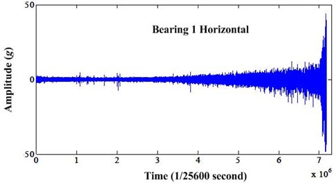
For training data, bearing lives varied from minimum life of 5,150 seconds to maximum life of 28,030 seconds. The truncated lives of testing bearings also varied with the minimum of 1,720 seconds and maximum of 23,020 seconds. Vibration measurements were performed every ten seconds and last 0.1 second. The training and testing data also included temperature measurements (with period 0.1 second). The sampling frequency of vibration signal is 25.6 kHz. The failure is defined as the amplitude of the vibration signal exceeding 20 g in the challenge explanation. This can be illustrated in Fig. 1 which denotes the whole degradation process of bearing 1 in first train group.
Fig. 1Vibration changing of bearing 1 depending of time
3. Prediction framework based on shock pulse method and frequency analysis
In this section, the fundamental theories of shock pulse method (SPM) and envelope analysis are given first. Then, new prediction method based on these two theories is proposed and the detail processes are presented.
3.1. Shock pulse method
The shock pulse method (SPM) [28] has been developed by SPM Instrument AB in early 1970s in Sweden. It is widely accepted as a quantitative method for tracking the degradation of bearings. It is based on the fact that when a roller passes a damaged area of raceway, an impulse of vibration is generated. The bearing condition can be indicated by the maximum normalized shock (MNS) value (dB). It is defined as:
where denotes the rotating speed of bearing, and is the inner diameter. is the shock value, which can be calculated by demodulation of bearing vibration signals. According to the experience, SPM corporation divided the bearing degradation process into three states [28]:
Healthy state: 020;
Weak fault state: 2035;
Heavy fault state: 3560.
These condition zones were empirically established by testing bearings under variable operating condition in the early 1970s. For over 44 years, based on these condition zones, SPM has been very successfully used to detect and track the degradation process of bearings. This method has been widely accepted in industries.
Using MNS value as a health indicator is very beneficially. In reality, same type bearings may be working under different operating condition and one bearing also may be working under varying conditions. Many health indicators only can reflect the bearing degradation process under constant operating conditions. This will affect the performance of prediction methods. On the contrary, MNS value will not be affected by operating conditions and can track the bearing degradation well. In addition, because of the generally used condition zones, all the life data of same type bearing can be used to train the prediction model. As a result, the model will have better performance.
3.2. Frequency analysis
Sometimes, the indicators of bearing life data sets are non-trendable. For new bearings, the health indicators are usually very flat in their early stages. However, we do not know how long the early stage will last and this makes the RUL prediction impossible. In order to solve the problem, another way of analysis should be used. As a rule, bearing faults cannot be detected by low-frequency vibration parameters until damage is quite severe. The reason for this is that when the roller passes over a damaged area of the race, a shock pulse is created which can be detected only in the high-frequency range at first. Then, when the faults progress, the resonance frequency will vary. Therefore, we can detect the incipient fault through observing the frequency variation.
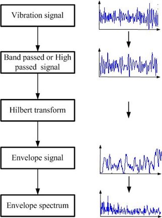
Generally, envelope analysis can be used to demodulate the signal and enable the fault detection easier. When bearing has some faults, such as: inner race defect, outer race defect, roller defect and cage defect, one can find the relevant fault frequencies. With the faults progressing, the high harmonics of fault frequencies will be found in the envelope spectrum. So, it is sure that the bearing faults also can be found by observing the frequency variation in the envelope spectrum. The calculation of MNS value and frequency analysis used to detect the state change point all were based on the processing of envelope spectrum. So, the steps of envelope analysis are given in Fig. 2.
Fig. 2The diagram of envelope analysis
3.3. Proposed prediction method
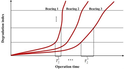
Bearings always experience several degradation states from new to failure. Sometimes, we can assume that the sojourn times of degradation states of different bearing are proportional. For example, same states should have same percentages in their full lives. It can be defined as:
where denotes the sojourn time of state of bearing . This can be further illustrated in Fig. 3.
Under this assumption, an example can be given. Suppose there are two bearings of same type. The life of bearing 1 is 1,000 hours. The life of bearing 2 is 3,000 hours. If all these two bearings have three degradation states, we say same degradation state have same percentage in the total life, respectively. For bearing 1, the sojourn times of three degradation states are 600 hours, 300 hours and 100 hours, respectively. Similarly, for bearing 2, the sojourn times of three degradation states are 1,800 hours, 900 hours and 300 hours, respectively. State 1 of bearing 1 has 60 % of the total life. And state 2 of bearing 2 also has 60 % of the total life. They are same. This is only the rational case to explain the Eq. (2).
Fig. 3Schematic diagram of the degradation process of three bearings
Therefore, if the state change point can be detected in new bearing, its RUL can be estimated according to the life percentage of previous state which can be calculated in history data. When the fault progresses and enter into next state, the RUL can be updated. However, the state number of same type bearings may be different. Some may experience two states and others may experience three states. This must be identified according to the specific characteristics of data. For the RUL prediction of challenge data, we will use SPM combined with frequency analysis to determine the values in Section 4. The key steps of proposed prediction method are as follows:
1) The degradation indicator – MNS values of training data are extracted. This degradation indicator has two functions. One is to define the failure threshold. The other is to find the degradation state change point.
2) Sometimes, the MNS value has not degradation trend and cannot find any information for the degradation state change point. So, in this case, frequency analysis of the envelope spectrum of total life is needed to detect the degradation state change point. Frequency variation information of the training data also are extracted.
3) After MNS values and frequency variation information have been extracted, the total lives and the sojourn times of each degradation state of bearings used for training can be determined. If the MNS value and frequency variation information both can be used, we use the mean value of RULs determined by these two methods. If the MNS values are non-trendable, we only use the degradation sojourn time determined by frequency variation information.
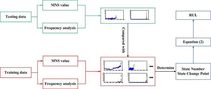
4) When a new bearing is working and goes into the degradation process, the MNS value and the frequency variation information can be acquired. Once the degradation state change point was detected, the RUL of this bearing can be determined according to Eq. (2). In addition, except the state change point, the degradation state number also can be determined according to the characteristics of frequency variation information. This is the key step to determine which training data should be used to as a reference – two degradation states training data or three degradation states training data. The overall processes of RUL prediction can be depicted in Fig. 4.
In engineering application, the operating conditions of bearing are very complex. However, MNS value extracted using shock pulse method is very robust and not sensitive to the varying operating condition. In addition, this method is widely used in many factories. On the other hand, not all the degradation processes of bearings can extract trendable MNS values. In this case, as a supplementary means, frequency variation information can be used to detect the degradation state change point. So, actually speaking, proposed method in this paper is very robust to process some engineering cases.
Fig. 4RUL prediction processes of proposed methods
4. Data analysis and discussion
Because of the page limit, only the first group bearing data are analyzed in this paper. According to SPM theory depicted in Section 3.1, MNS values of seven bearing lives can be calculated and illustrated in Fig. 5. It can be seen that degradation processes of bearing 1 and 3, bearing 2 and 4 are similar. However, for bearings 5-7, we cannot extrapolate the state change points only observing the MNS values. The degradation processes may be similar to bearing 1 or bearing 2. This makes the RUL prediction impossible.
The failure of bearing is claimed when the amplitude of vibration signal exceeds the threshold of 20 g. This is a vague statement because some amplitudes exceeds the threshold but some others not. Therefore, the failure threshold should be redefined according to the new degradation feature. For the bearings 1 and 3, it can be seen from Fig. 5 that the MNS values of horizontal direction have more obvious trend than the vertical direction. So, the MNS values of horizontal direction are used to define the failure threshold. The maximum MNS value of bearing 1 is selected as the failure threshold denoted as . It can be seen in Fig. 6. In the figure, red crosses mean the degradation state change point.
This is the first training data set. It can be seen that bearing 1 has three degradation states. The transition point from state 1 to state 2 is at about time 1,200 and state 2 to state 3 is at about time 2,747. The maximum MNS value of bearing 2 is not exceed the failure threshold as shown in Fig. 7. So, we need to recalculate the life of bearing 2. The straight line can be used to fit the MNS value until it exceeds the failure threshold. The results of and are 0.12 and 14.09. They are calculated using linear fitting function of Matlab. Similarly, the bearing 2 has experienced two degradation states. The transition point from state 1 to state 2 is at about time 814. The readjusted life of bearing 2 after fitting is 943.
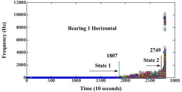
In addition, we should investigate the frequency domain characteristics of these two bearings. In this paper, high pass filter is used for envelope analysis. The band pass frequency is 30 times of rotating frequency. Their frequency variations of whole life after envelope analysis can be seen in Figs. 8 and 9. From the frequency variation, we can find different state change point. The MNS value and the frequency analysis can be combined to predict the RUL and use the mean value as the predicted RUL. The prediction process can be divided into three steps. First, we should attempt to find the state change point in the MNS value and compare testing data with training data to find the similar one. If this is possible, both MNS value analysis and frequency analysis can be used to extrapolate the RUL. Second, if one cannot find the state change point in the MNS value, the frequency analysis should be used to find the state change point. Finally, we must determine the most probable degradation state number through the frequency characteristics analysis. It should be mentioned that the color codes of bubble markers in the following figures denotes the amplitude of the frequency. From blue to red, it denotes the bigger amplitude variation.
Fig. 5MNS values of first group bearings
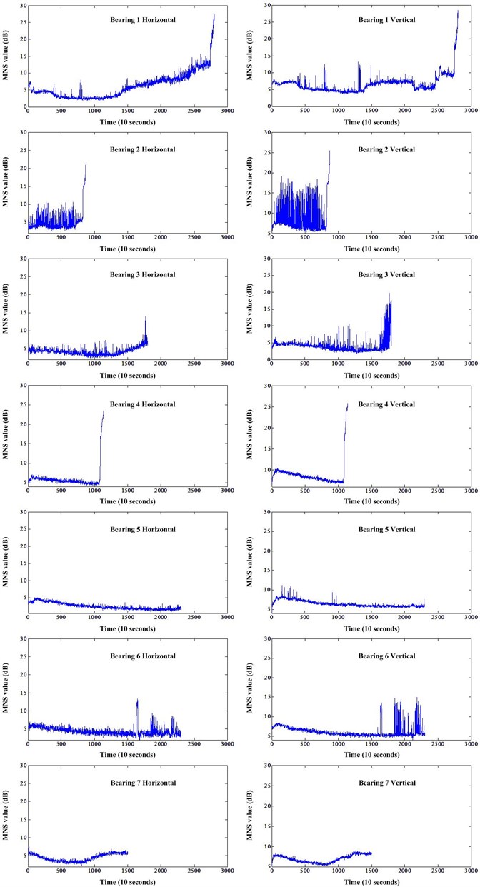
Fig. 6Horizontal MNS value of bearing 1
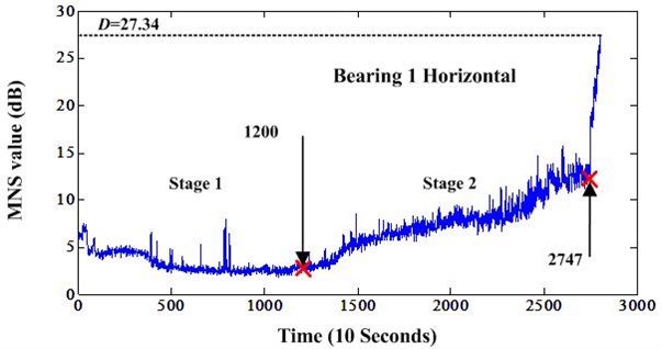
Fig. 7Horizontal MNS value of bearing 2
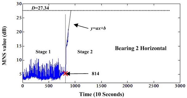
Fig. 8Frequency variation of bearing 1 after envelope analysis
Next, we start to analyze the testing data. Fig. 5 shows that bearings 1 and 3, bearings 2 and 4 have similar trend. And, the state change point can be reflected by both the MNS value and frequency variation information. So, both these information can be used to predict the RUL of bearings 3 and 4. Then, the mean value is selected as the final RUL. The frequency variations of bearings 3 and 4 are illustrated in Figs. 10 and 11.
Then, we can continue to analyze the truncated data of bearings 5-7. Fig. 5 shows that the MNS values of these three bearings are non-trendable. We cannot find the change points from these MNS values information. So, frequency analysis can be used to track the state change point. The frequency variation information of bearings 5-7 are depicted in Figs. 12-14. The horizontal direction frequency variation of bearing 5 is vague to determine the state change point. So, we need to observe the frequency variation of vertical direction. It is depicted in Fig. 15. Synthesizing these two frequency variation information, the final point can be considered as the state change point. And we can see that the change point of bearings 6 and 7 can be easily detected using horizontal direction frequency variation information.
Fig. 9Frequency variation of bearing 2 after envelope analysis
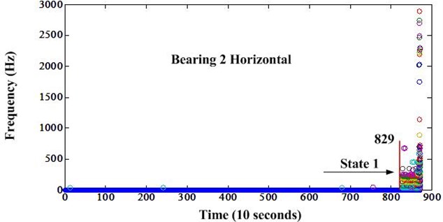
Fig. 10Frequency variation of bearing 3 after envelope analysis
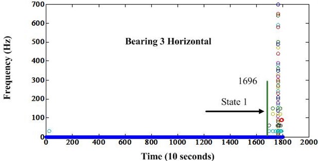
Fig. 11Frequency variation of bearing 4 after envelope analysis
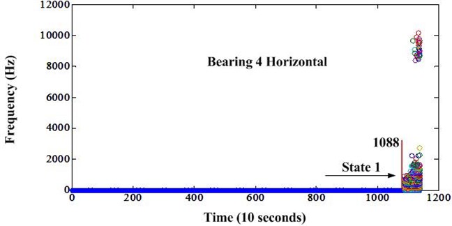
Fig. 12Frequency variation of bearing 5 after envelope analysis
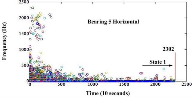
Fig. 13Frequency variation of bearing 6 after envelope analysis
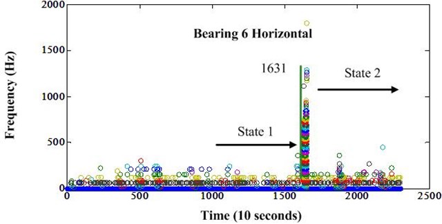
Fig. 14Frequency variation of bearing 7 after envelope analysis
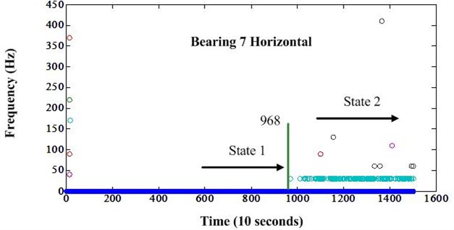
However, training data has two cases. There are two degradation states for bearing 2 and three degradation states for bearing 3. Therefore, the remaining bearings of testing data sets also have two or three degradation states. So, when the state change point has been detected, we need to know two things. One is which state it will transits to? Another is how many states this bearing has? If we know these information, we can predict the RUL easily according to the training data. For bearings 3 and 4, we can know bearing 3 has three states and bearing 4 has two states. The Figs. 10 and 11 also showed important information: if the frequency range at first change point is about 0-1000 Hz, it denotes this bearing has three states and the change point is the transition from state 1 to state 2; if the frequency range at first change point is about 0-2000 Hz or bigger than this range, it states that this bearing has two states and the change point is the transition from state 1 to last state. According to this theory, the states of all testing bearings can be determined. Bearing 3 has three states, bearing 4 has two states, bearing 5 has two states, bearing 6 has three states and bearing 7 has three states. Finally, the RUL of testing bearings can be determined according to Eq. (2) in Section 3.3 and the state sojourn times of training data. For bearing 7, the predicted RUL according to the sojourn time of state 1 is negative. This is not practical. So, the sojourn time of state 2 is used for RUL prediction. The results are displayed in Table 1 and compared to the results in reference [23]. It shows that the performance of proposed methods is better than methods used in [23].
s
Fig. 15Vertical direction frequency variation of bearing 5 after envelope analysis
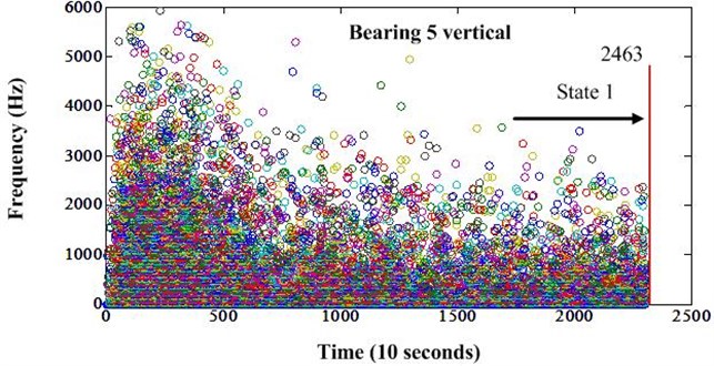
Table 1Comparison of RUL prediction and ground truth of group 1 data
Bearing ID | Current life (10 s) | RUL truth (10 s) | RUL prediction (10 s) | RUL in [23] |
Bearing 3 | 1802 | 573 | 1004 | 49 |
Bearing 4 | 1139 | 289 | 106 | 1 |
Bearing 5 | 2302 | 161 | 313 | 49 |
Bearing 6 | 2302 | 146 | 226 | 49 |
Bearing 7 | 1502 | 757 | 116 | 49 |
Because of small amount of training data, the sojourn times of each degradation state cannot reflect the real percentage which they belong to the whole life. If more training data can be obtained, the performance of RUL prediction will be better. Second, for the bearings 3, 6 and 7, when they continue deteriorate, the second state change point will be detected. Then, more information can be used to predict the RUL and achieve better results. Third, it is possible that there is more feasible proportional relationship between state sojourn times than the direct ratio.
5. Conclusions
In this paper, SPM and frequency analysis are combined to analyze the 2012 PHM challenge data. The MNS value extracted according to SPM theory is less sensitive to the operating condition, which enables the prediction of the bearing RUL possible in varying operating condition. When the MNS value is non-trendable, frequency analysis can be used to detect the degradation state change point. It is assumed that the state sojourn times are proportional for different bearings. So, the RUL can be predicted when the state change point is detected. This method is more robust than some time series methods. The results of challenge data analysis demonstrate the effectiveness of proposed method. In the challenge data, bearings only have two or three degradation states because this experiment is accelerated test. There may be many degradation states for normal working bearing. So, the RUL can be adjusted when new state change point has been detected. As a future study, the degradation process will be investigated by combining the frequency analysis and machine learning methods.
References
-
Jardine A. K. S., Lin D. M., Banjevic D. A review on machinery diagnostics and prognostics implementing condition-based maintenance. Mechanical Systems and Signal Processing, Vol. 20, Issue 7, 2006, p. 1483-1510.
-
Zhang X. D., Xu R., Kwan C., Liang S. Y., Xie Q. L., Haynes L. An integrated approach to bearing fault diagnostics and prognostics. American Control Conference, 2005, p. 2750-2755.
-
Kaiser K. A., Gebraeel N. Z. Predictive maintenance management using sensor-based degradation models. IEEE Transactions on Systems, Man and Cybernetics – Part A: Systems and Humans, Vol. 39, Issue 4, 2009, p. 840-849.
-
Gebraeel N. Z., Elwany A., Pan J. Residual life predictions in the absence of prior degradation knowledge. IEEE Transactions on Reliability, Vol. 58, Issue 1, 2009, p. 106-117.
-
Widodo A., Yang B. S. Machine health prognostics using survival probability and support vector machine. Expert Systems with Applications, Vol. 38, Issue 7, 2011, p. 8430-8437.
-
Tobon-Mejia D. A., Medjaher K., Zerhouni N., Tripot G. A data-driven failure prognostics method based on mixture of gaussians hidden Markov models. IEEE Transactions on Reliability, Vol. 61, Issue 2, 2012, p. 491-503.
-
Dong M., He D. A segmental hidden semi-Markov model (HSMM)-based diagnostics and prognostics framework and methodology. Mechanical Systems and Signal Processing, Vol. 21, Issue 5, 2007, p. 2248-2266.
-
Dong M., Peng Y. Equipment PHM using non-stationary segmental hidden semi-Markov model. Robertics and Computer-Integrated Manufacturing, Vol. 27, Issue 3, 2011, p. 581-590.
-
Peng Y., Dong M. A prognosis method using age-dependent hidden semi-Markov model for equipment health prediction. Mechanical Systems and Signal Processing, Vol. 25, Issue 1, 2011, p. 237-252.
-
Liu Q. M., Dong M., Peng Y. A novel method for online health prognosis of equipment based on hidden semi-Markov model using sequential Monte Carlo methods. Mechanical Systems and Signal Processing, Vol. 32, 2012, p. 331-348.
-
Wu B. R., Tian Z. G., Chen M. Y. Condition based maintenance optimization using neural network based health condition prediction. Quality and Reliability Engineering International, Vol. 29, Issue 8, 2013, p. 1151-1163.
-
Kim H. E., Tan A. C. C., Mathew J., Choi B. K. Bearing fault prognosis based on health state probability estimation. Expert Systems with Applications, Vol. 39, Issue 5, 2012, p. 5200-5213.
-
Tian Z. G., Liao H. T. Condition based maintenance optimization for multi-component systems using proportional hazards model. Reliability Engineering and System Safety, Vol. 96, Issue 5, 2010, p. 581-589.
-
Tran V. T., Pham H. T., Yang B. S., Nguyen T. T. Machine performance degradation assessment and remaining useful life prediction using proportional hazard model and support vector machine. Mechanical Systems and Signal Processing, Vol. 32, 2012, p. 320-330.
-
Zhang X. H., Kang J. S., Jin T. Degradation modeling and maintenance decisions based on Bayesian Belief Networks. IEEE Transactions on Reliability, Vol. 63, Issue 2, 2014, p. 620-633.
-
Wang W. B., Carr M. J. A stochastic filtering based data driven approach for residual life prediction and condition based maintenance decision making support. International Conference on Prognostics and Systems Health Mangament, Macau, China, 2010, p. 1-10.
-
Wang W. B., Hussin B., Jefferis T. A case study of condition based maintenance modelling based upon the oil analysis data of marine diesel engine using stochastic filtering. Internatinal Journal of Production Economics, Vol. 136, Issue 1, 2011, p. 84-92.
-
Carr M. J., Wang W. B. Modeling failure modes for residual life prediction using stochastic filtering theory. IEEE Transactions on Reliability, Vol. 59, Issue 2, 2010, p. 346-355.
-
Sun J. Z., Zuo H. F., Wang W. B., Pecht M. G. Application of a state space modeling technique to system prognostics based on a health index for condition-based maintenance. Mechanical Systems and Signal Processing, Vol. 28, 2012, p. 585-596.
-
Feng L., Wang H. L., Si X. S., Zou H. X. A state-space-based prognostic model for hidden and age-dependent nonlinear degradation process. IEEE Transactions on Automation Science and Engineering, Vol. 10, Issue 4, 2013, p. 1072-1086.
-
Nectoux P., Gouriveau R., Medjaher K., Ramasso E., Morello B., Zerhouni N., Varnier C. An experimental platform for bearings accelerated life test. IEEE International Conference on Prognostics and Health Management, Denver, USA, 2012.
-
Boškoski P., Gašperin M., Petelin D. Bearing fault prognostics based on signal complexity and Gaussian process models. IEEE International Conference on Prognostics and Health Management, Denver, USA, 2012.
-
Wang T. Y. Bearing life prediction based on vibration signals-A case study and lessons learned. IEEE International Conference on Prognostics and Health Management, Denver, USA, 2012.
-
Sutrisno E., Oh H., Vasan A. S. S., Pecht M. Estimation of remaining useful life of ball bearings using data driven methodologies. IEEE International Conference on Prognostics and Health Management, Denver, USA, 2012.
-
Porotsky S. Remaining useful life estimation for systems with non-trendability behavior. IEEE International Conference on Prognostics and Health Management, Denver, USA, 2012.
-
Gu H. Q., Zhao J. M., Zhang X. H. Hybrid methodology of degradation feature extraction for bearing prognostics. Eksploatacja I Niezawodnosc – Maintenance and Reliability, Vol. 15, Issue 2, 2013, p. 195-201.
-
Challenge Data Sets. http://www.femto-st.fr/en/Research-departments/AS2M/Research-groups/ PHM/IEEE-PHM-2012-Data-challenge.php.
-
The shock pulse method for determining condition of anti-friction bearings. SPM Technical Information, Sweden, SPM Instruments AB.
About this article
This program is partially supported by Chinese Government Programs under Grant No. 51327020304.
