Data transfer of non-matching meshes in a common dimensionality reduction space for turbine blade

1. Introduction

Fluid structure interaction (FSI) problems are characterized by the interaction of fluid and structure, and fluid pressure will make the structure move. Simulation of this class of problems involves two different disciplines, computational fluid dynamics (CFD) and computational structure mechanics (CSM). In stead of solving the whole system of fluid and structure all at once, decomposition method or partitioned coupling method is widely used, as the available CFD and CSM solvers are developed separately. Decomposition method separates FSI system along the natural interface of fluid and structure. So, data transfer is needed to re-couple the fluid and structure domains. Pressure loads is needed to be transmitted from the fluid side of the fluid-structure interface to the structure nodes on the same interface, and the motion of interface meshes also is needed to be transmitted to the fluid mesh points [1-2].

Commonly, at interface, the CFD and CSM meshes are non-matched meshes which is hardly impossible to get the accurate solution between the non-matched meshes. Thus, data transfer have a very important position on how to get the accuracy of calculation between the interface of CFD and CSM meshes. Just because of this, a number of methods [2-5], such as interpolation method and projection method, have been carried out to transfer data across non-matching meshes.

Interpolation method is a direct way to transfer data, obtain data from the closest points of data source mesh through some nearest neighbor interpolation function, by spline function, or by radial basis functions [3-6]. This method is simple and direct. However, only when the structure and fluid domains have fine interface meshes, the interpolation method can get good results. However, when meet the coarse non-matching meshes with gap and overlap, the discrete error of CFD and CSM will show up sharply in the interpolation results and will get worse transfer results.

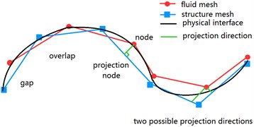
Another way to transfer data is the method of projection mentioned in [6-12]. To obtain information from the data source, a node will be orthogonal projected onto the source mesh and the information of the projected node will be calculated in that mesh [6-7], shown as in Fig. 1.

However, these projection methods mentioned above often suffer from lacking of accuracy in transferring loads across non-matched meshes [8-9]. Because in practical problems, the non-matching meshes will lead to discrepancy in the calculated normal and area of different disciplines and then no-accurate interpolation result [4, 9] will be resulted. To overcome this problem, a common refinement mesh method is proposed in the interface [8, 10-12], and the interface meshes are subdivided into ‘subelements’ to construct a common refinement mesh for the fluid and structure meshes and data is then transferred on the ‘subelements’. Because of many fine meshes are used, this method enables robust and accurate numerical data transfer result can be got. However, the common-refinement mesh method can be mainly focused on two disciplinary meshes. If a common refinement meshes are needed in more disciplines or dynamics mesh problems, the calculation duty will increase more largely.

Fig. 1Scheme of projection method

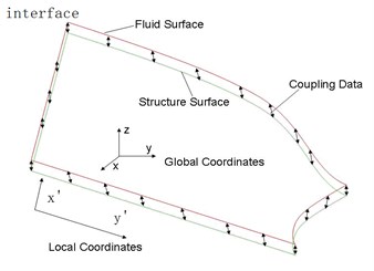
To illustrate the gap and overlap occur in the fluid and structure meshes clearly, a coupling curved interface of fluid and structure is created and is shown in Fig. 2. In the Fig. 2, the difficult point of interpolation comes from the gap and overlap between the fluid and structure meshes. In the present data transfer methods, the data can only be transferred among meshes, thus, the accuracy is limited by the mesh size. From another point of view, the meshes belong to interface, but the interface does not belong to the meshes, thus, the data will be transferred on physical interface, and the data will not be transferred in the interface meshes. In the case of the data is interpolated on physical interface, it will be free of non-matched mesh errors, and the gap and overlap between meshes will be disappeared. However, during interpolation, there is no information about the physical interface except the approximation will be represented by meshes. So, in order to get more accurate solution, the interface from these meshes was reconstructed in [3, 13].

Fig. 2Coupling curved interface of fluid and structure

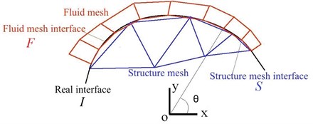
And one thing must be noticed is that the interfaces between fluid and structure are quasi-3D (quasi-2D) surfaces, while the interfaces are not real 3D (2D) objects [14]. If data is transferred in a dimensionality reduction projection space, the interface need not to be reconstructed. For example, if local coordinate system is defined for the curved interface shown in Fig. 2, from $\theta$ point of view, there will be no gap between fluid and solid meshes, the interpolation can be done on coordinate $\theta$. And there is no need to rebuild the physical interface. Because all meshes and nodes will be projected on the space, it can also be called dimensionality reduction (common projection) space. Obviously, if the data is transferred in 2D (1D) space, its searching and interpolation will be faster than directly transferred in 3D (2D) space.

In the manuscript, a new method which the data is transferred in dimensionality reduction [15-17] space of interface surface is proposed. In the new method, local coordinates system is set to project interface surface into reduce dimensionality space. For illustrating on how to use local coordinates system to reduce dimensionality, the temperature of a turbine blade is transferred in common projection space are given as an example.

2. Numerical considerations

The method in the manuscript provided common dimensionality reducion space for interface and transfer data in the common space. By reducing dimensionality, 3D coupling data interpolation can be done in 2D space and 2D interpolation can be done in 1D space. In widely used data transfer method, data points may be wrongly used in data transfer for coupling interface of thin structure, such as blade or wing. Whereas reducing dimensionality of interface during data transfer as the method provided in this paper, the coupling data can be interpolated directly in curved local coordinates.

Is provided to reduce the dimensionality of coupling interface. Compared to projection methods which were used widely in the surface parameterization of CAG (computer aided geographic), no searching and interpolation are needed in the local coordinate projection method which will result in considerable savings in computational time and costs in the data transfer.

2.1. Define common projection space by local coordinates

In the following section, the coupling interface can be classified into 3 types, and different coordinates system can be used to define projection for the coupling interface. Normally, for simple surface, the local coordinate projection can be defined directly. Whereas, in the practical engineering problem, we always meet the complex surface, then,we can not define the local coordinate projection directly in such complex surface. Like such complex surface, we can divide the complex surfaces into several simple surfaces and then define the projection through local coordinate for each of divided simple surfaces.

The example for different surface is listed as follows. And in the local coordinates, $u$ and $v$ are projection coordinate, respectively; $\theta$ is angle coordinates; $x$, $y$, $z$ are 3D coordinate, separately.

1) For cylinder surface or blended surface in one direction, a cylindrical coordinates system can be set as Fig. 3. Projection of cylinder surface or blended surface can be defined as Eq. (1). The dimensionality normal to surface is reduced by the projection:

1

$\left\{\begin{array}{ll}u=\theta ,& -\pi \le \theta <\pi ,\\ v=z,& 0<z\le L.\end{array}\right.$

Fig. 3Cylindrical coordinates for one-direction curved interface

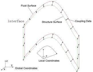
Fig. 4Local spherical coordinates for two-direction curved interface

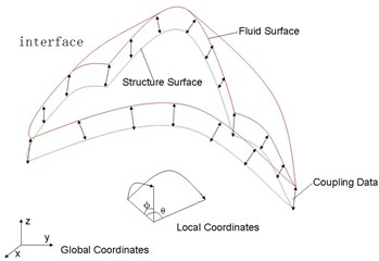
2) Local spherical coordinates system for sphere surface or surface blending in two directions is shown in Fig. 4. Projection for sphere surface or surface blending in two directions is defined as Eq. (2). The dimensionality normal to surface is reduced by the projection:

2

$\left\{\begin{array}{ll}u=\theta ,& -\pi \le \theta <\pi ,\\ v=\phi ,& 0<\phi \le \frac{\pi }{2}.\end{array}\right.$

3) For flat surface, the local coordinates system is defined parallel to surface as shown in Fig. 5. And the projection for flat interface is defined as Eqs. (3). The dimensionality normal to surface is reduced by the projection:

3

$\left\{\begin{array}{l}u=x^{\mathrm{\text{'}}},\\ v=y^{\mathrm{\text{'}}}.\end{array}\right.$

Fig. 5Local Cartesian coordinates for flat interface

2.2. Data transfer in common projection space

The steps on how to transfer the temperature data of the coupling interface surface of blade in dimensionality reduction space is illustrated. The scheme of the steps are shown in the Fig. 6.

Fig. 6Scheme of steps on temperature data transfer process in common projection space

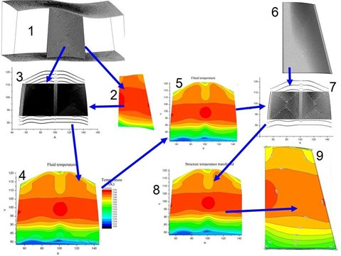
In Fig. 6, the meaning of the number from 1-9 are shown as Table 1.

In the Fig. 6, the temperature data of fluid (2) is needed to be transferred to the structure model (6) as temperature load. Firstly, according to the geometry shape of the coupling interface surface of blade, a local cylindrical coordinates system is defined, and the fluid interface nodes(1) are projected in common plane space (3) according the local cylindrical coordinates system. According to the projection corresponding relationship of nodes, the node temperature in (2) is assigned to the projected nodes in the common plane space (3), where the temperature distribution (4) is formed. Temperature distribution can be fitted in common space by proper function. The nodes of the structure interface surface can be mapped to the projected structure nodes (7) in the common space. The fitting data in (5) is then interpolated to the projected structure nodes of (7). The temperature data (8) of the structure nodes in common space is got. According to the corresponding relationship between the projected nodes and the structure nodes in 3D space, the temperature data in (8) can be transferred to the structure nodes of coupling interface of the 3D blade surface.

Table 1List of the meaning of the number in Fig. 6

No.	Indication
1	Fluid mesh
2	Fluid temperature
3	Fluid nodes of interface surface projected in common space
4	Fluid temperature in common space
5	Fitted fluid temperature in common space
6	Structure mesh
7	Structure nodes of interface surface projected in common space
8	Node temperature of structure interface interpolated from fitted fluid temperature in common space
9	Transferred temperature of structure

3. Examples: Temperature transfer for a turbine blade

In this section, the proposed method mentioned above is used to deal with the temperature data transfer for a turbine blade.

3.1. Projection method for the blade interface

A turbine blade is shown in Fig. 7. In practical engineering problem, the temperature data and pressure data are needed to be transferred together. But as an example, for illustrating clearly, only the temperature data is transferred in this paper.

Fig. 7Define local coordinates frame for blade interface

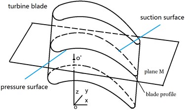
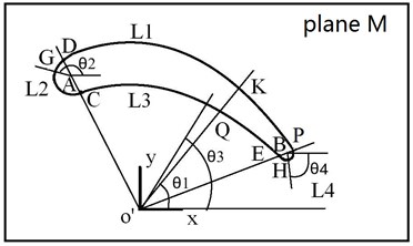
Fig. 8Blade profile at cutting plane M

The proposed method mentioned above is used to transfer the temperature data of the blade. In the method, local coordinates is set up for projection. In the Fig. 7, the interface of the blade is column somewhat, the cylinder coordinates is used here. But, if cylinder coordinates is used directly, the projection will be not monotonic, that is, no matter where we set the local coordinates origin, there will be two points of interface surface for an angle coordinates. Thus, we break the interface surface into 4 pieces and define the local coordinates and the projection for each piece.

In Fig. 7, define a local coordinates system $x$-$y$-$z$ at the middle of the blade in longitude direction, off the pressure surface of the blade. Define the axis $x$ along the longitude direction of the blade; define the axis $z$ along the blade spanwise; define the axis $y$ vertical to the $x$-$z$ plane. Paralleling to plane $x$-$y$, makes a plane M. The intersection of the plane M and the interface surface will form a blade profile, as shown in Fig. 8.

In Fig. 8, the plane M and axis $z$ have an intersection point o'. At the plane M, making a line passing the point o' and the arc center A of the blade leading edge L2, the line o'A and the blade profile has two intersection point, C and D. Making a line passing the point o' and the arc center B of the blade trailing edge L4. The line o'B and the profile line have two intersection points, E and P. Then, the points, C, D, E, and P, divide the blade profile into 4 smaller lines, L1, L2, L3, and L4. Make a line Ko' which pass any point K of the line L1 and the point o'. Define the angle between line Ko' and axis $x$ as ${\theta }_1$. Make a line pass a point G of the line L2 and the arc center A, define the angle between the line GA and the axis $x\text{'}$ as ${\theta }_2$. Make a line passing a point Q of the line L3 and the point o', define the angle between the line Q o' and the axis $x\text{'}$ as ${\theta }_3$. Make a line pass any point H of the line L4 and the arc center B, the angle between the line HB and the axis $x\text{'}$ as ${\theta }_4$ is defined.

Move the plane M along axis $z$, a series of cut planes and blade profile are got. Then, each of the blade profile can be defined the similar local coordinates system and line pieces are got.

To any point in the blade profile, its projection local coordinates is illustrated. For a point at the line L1, a projection coordinates is defined as $u={\theta }_1$. For a point at the line L2, a projection coordinates is defined as $u={\theta }_2$. For a point at the line L3, a projection coordinates is defined as $u=u_1+180+(u_1-{\theta }_3)$, where $u_1$ is the ${\theta }_1$ value of the point D in the line L1. For a point at the line L4, a projection coordinates is defined as $u={\theta }_3$.

The projection coordinates $v$ of any cut blade profile along spanwise is defined to equal to $z$ of the cut plane M.

Then, the projection for the blade interface surface is given as follows Eq. (4):

4

$\left\{\begin{array}{l}u=\left\{\begin{array}{ll}{\theta }_1,& L_1,\\ {\theta }_2,& L_2,\\ u_1+180+\left(u_1-{\theta }_3\right),& L_3,\\ {\theta }_3,& L_4,\end{array}\right.\\ v=Z.\end{array}\right.$

The projection coordinates of the blade interface surface is set and can be used to reduce dimensionality of the interface surface and to transfer temperature data of the blade.

3.2. Temperature transfer result of turbine blade

3.2.1. Fitting temperature load of turbine blade in common space

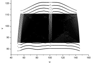
According to the method mentioned above, project the interface surface nodes of the fluid mesh (as shown in Fig. 9) into a common space, and the fluid nodes in common space (Fig. 10) is got.

Fig. 9Fluid mesh of blade

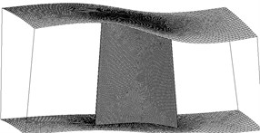
Fig. 10Fluid nodes projected into the defined common space

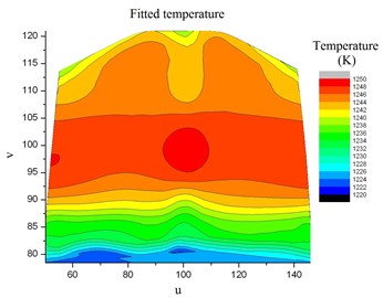
Project the corresponding fluid temperature of nodes of the turbine blade in Fig. 11 into the common space, and the fluid temperature distribution of the blade interface surface in the common space is shown in Fig. 12. Fitting the temperature data in the common space with bi-cubic B-spline, the fitted temperature distribution function is got as shown in Fig. 13. This function as temperature load will be interpolated to the structure meshes of the turbine blade.

Fig. 11Fluid temperature of the turbine blade

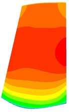
a) Suction surface

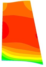
b) Pressure surface

Fig. 12Fluid temperature distribution in the common space

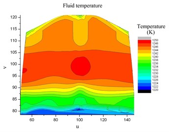
Fig. 13Fluid temperature fitted by bi-cubic B-spline in the common space

3.2.2. Interpolating temperature load in common space

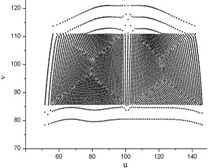
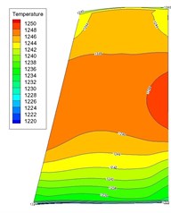
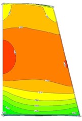
Project the structure nodes in Fig. 14 into the same common space in section 3.2.1, and then the projected nodes of structure interface of the turbine blade are shown in Fig. 15. In the common space, the temperature load of the structure nodes can be interpolated by the fitted bi-cubic B-spline function of fluid temperature. The interpolated temperature of the structure nodes in the common space is shown in Fig. 16. Then, the temperature of any blade structure node in 3D space can be got according to the interpolated temperature of its corresponding projected node in common space. At last, the result of the interpolated temperature load of the turbine blade is shown in Fig. 17.

Fig. 14Structure mesh

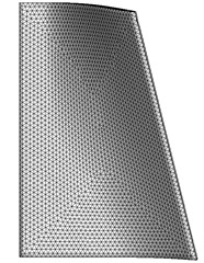
Fig. 15Structure nodes projected in the common space

3.2.3. Error discussion

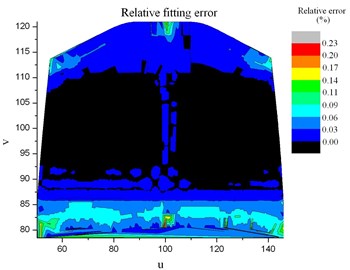
Compared the CFD temperature Fig. 10 and the transferred CSM result Fig. 17. The temperature of the blade is from 1220 K to 1250 K. It can be observed that the fluid temperature and the interpolated temperature of the turbine blade interface match well, which indicates the temperature transfer method is accurate. The absulate temperature transfer error in common space is shown in Fig. 18. The relative temperature transfer error in common space is shown in Fig. 19. From Fig. 18 and Fig. 19, it can be observed that the max absolute temperature transfer error is 2.8 K and the max relative transfer temperature error is 0.23 %. The temperature transfer method is accurate numerically. Generally the proposed method described above is accurate.

Fig. 16Structure temperature interpolated by bi-cubic B-spline in the common space

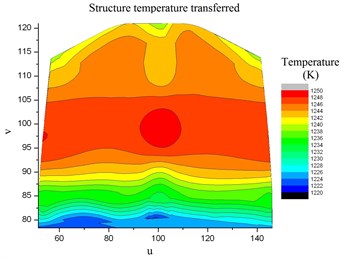
Fig. 17Interpolated tempereature load of turbine blade

a) Suction surface

b) Pressure surface

Fig. 18Absolute fitting error of the fluid temperature

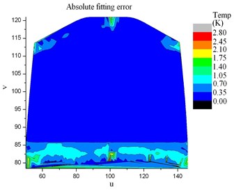
Fig. 19Relative fitting error of the fluid temperature

4. Summary

A new method is presented to transfer the temperature of turbine blades from the CFD result to the CSM model with non-matching meshes. The method described above is also applicable to transfer of pressure, displacement and velocity as well.

In the method, local coordinates system is carried out to reduce dimensionality. By the means of dimensionality reduction, 3D interpolation can be done in 2D space. The method provided in this paper has been validated in section 3, which can be used for coupling interface of thin structure directly in curved local coordinates.

For illustrating how to use local coordinates system to reduce dimensionality, the temperature of a turbine blade is transferred in common projection space are given as an example. Compared to projection methods widely used in the surface parameterization of CAG (computer aided geographic), the local projection method provided in this paper is much more easier for mapping nodes of coupling interface and can accelerate data transfer process. The method in example is designed mainly for turbine blade and wing. For other kind of geometry excluded blade and wing in the manuscript, the projection method used in the data transfer method described above is needed to be modified.

Compared to Ref. [1-2, 8, 10, 11], the method provided here has no special requirement of refining the meshes of interface surface to get accurate data transfer. The complex 3D FSI data transfer problem is simplified and the error is minimized induced by non-matching meshes.