A bearing fault detection method based on compressive measurements of vibration signal

1. Introduction

In the field of condition monitoring and fault diagnosis of rotating machinery, it is always necessary to monitor the component uninterruptedly for a long period of time. This process will generate masses of original data which would burden the storage and transmission. For the storage and transmission issue of vast amounts of vibration data, the general strategy can be described as follows. First we should sample the analog signal in the frame of Shannon sampling theory and acquire the original digital signal. Data can be compressed in appropriate ways such as space transformation and then we can acquire small amount of compressed data [1]. What we need to save and transmit should be the compressed data. In data analysis, we can decode the compressed data we saved to recover the original vibration data and implement fault detection and diagnosis etc. with relevant available methods.

In the process of signal sampling and compressing mentioned above, what we transmitted or saved should be a small part of the original data we sampled. The majority of the original data would be dropped, which should be an enormous waste of resources. Since the signal can be compressed, we should consider whether we can acquire the compressed data directly and omit much data contained little useful information at the same time. This idea is the rudiment of compressed sensing (CS). In 2006, Candès proved in mathematic principle that the original signal could be reconstructed using parts of its Fourier transform coefficients, which should be the theoretical foundation of compressed sensing [2]. Then Donoho and Candès et al proposed the concept of compressed sensing formally based on the related work [3, 4]. The main process of CS can be divided into two steps. First, we can acquire the non-adaptive linear projections (or measurements) of the original signal in compressed sampling way. Then we can reconstruct the original signal directly with these measurements in appropriate recovery algorithms [5-7]. Taking one-dimensional signal for example, the comparison of traditional signal compression with compressed sensing is shown in Fig. 1.

Fig. 1Comparison of traditional signal compression a) with compressed sensing b)

a)

b)

In the frame of compressed sensing, the original signal should be reconstructed first, and then fault can be detected with the recovered signal. Since the original signal can be recovered from the compressive measurements, then we should believe that these measurements should carry or contain enough information of the original signal. If the faults can be detected or diagnosed with the original signal, then the detection and diagnosis should also be achieved with the compressive measurements directly [8].

The bearing is one of the most commonly used but also the most vulnerable parts of rotating machinery equipment. It is also a failure-prone component due to the abominable working condition in addition to high speed and heavy load. Once failure, it will threaten the safe operation of the equipment, so it is necessary to monitor the bearings status and identify the fault in time [9]. The bearing faults can be characterized by the existence of shock pulses in vibration signals. In the time domain, the mean value and variance etc. of the vibration signal will change owing to the shock. While in the frequency domain, the shocks will enhance the high-frequency parts so that the energy distribution of the signal changes. According to these characteristics, we can achieve bearing fault detection based on the changes of the energy distribution in frequency domain. If we can collect fewer compressive measurements directly which contain the energy distribution information of current signal, then it is possible to achieve bearing fault detection using these measurements. Therefore, a new method focused on how to achieve bearing fault detection using small amount of compressive measurements directly is proposed in this paper.

The rest of this paper is organized as follows. In Section 2, we introduce the theory of compressed sensing. The bearing fault detection method based on compressed sensing is proposed in Section 3. The experimental tests are given in Section 4. Finally, the conclusions are drawn in Section 5.

2. Compressed sensing

For a signal $\mathbf{x}\in {\mathbf{R}}^N$, as described above, in the frame of CS we should acquire the linear projections of signal $\mathbf{x}$ first. The process of projecting can be converted into an observation matrix $\mathrm{\Phi }$: $M$×$N$ ($M<N$), and each row of matrix $\mathrm{\Phi }$ can be regarded as a sensor that multiplies with the signal and acquires parts of information of the signal. We can execute compressive measuring to $\mathbf{x}$ as:

Then we can acquire the linear measurements (or projections) $\mathbf{y}\in {\mathbf{R}}^M$. If $\mathbf{x}$ can be recovered from $\mathbf{y}$, it means that these fewer linear projections contain enough information to recover the signal $\mathbf{x}$, in which case the compressed sensing can be achieved. According to linear algebra theory, Eq. (1) should have infinitely many solutions and we can’t recover original signal $\mathbf{x}$ uniquely from measurements $\mathbf{y}$ when$\mathrm{}M<N$. However, if $\mathbf{x}$ is sparse (meaning that there only has a few non-zero elements in x), the number of unknowns will be reduced greatly, and this will make it possible to recover $\mathbf{x}$ from $\mathbf{y}$.

Actually, most nature signals are not sparse in general, while they can be represented sparsely with proper ways such as orthogonal transformation. If expanding $\mathbf{x}\in {\mathbf{R}}^N$on some orthogonal basis ${\left\{{\mathbf{\psi }}_i\right\}}_{i=1}^N$, where ${\mathbf{\psi }}_i$ is a $N$-dimensional column vector, we can get:

where the coefficient ${\mathrm{\theta }}_i=〈\mathbf{x},{\mathbf{\psi }}_i〉={\mathbf{\psi }}_i^T\mathbf{x}$, and Eq. (2) can be transferred into a matrix form as:

where $\mathrm{\Psi }=\left[{\psi }_1,{\psi }_2,{\dots ,\psi }_{\mathrm{N}}\right]\in {\mathbf{R}}^{N\times N}$ is defined as dictionary matrix, and expansion coefficient is $\mathrm{\Theta }={\left[{\mathrm{\theta }}_1{,\mathrm{\theta }}_2{,\dots ,\mathrm{\theta }}_{\mathrm{N}}\right]}^T$. Suppose that the coefficient vector $\mathrm{\Theta }$ is $K$-sparse on basis $\mathrm{\Psi }$, i.e. there has $K$ non-zero elements in $\mathrm{\Theta }$ and $K\ll N$, then $\mathrm{\Theta }$ can be entitled as sparse representation coefficient of $\mathbf{x}$ on dictionary matrix $\mathrm{\Psi }$. Taking Eq. (3) into Eq. (1) and denoting $\mathbf{A}=\mathrm{\Phi }\mathrm{\Psi }$, then we can get:

The matrix form of compressive measurements can be represented in Fig. 2. Considering that $\mathrm{\Theta }$ is sparse, the unknowns in Eq. (4) will be reduced greatly so that it is possible to recover $\mathrm{\Theta }$ from $\mathbf{y}$. In order to recover sparse signal, Candès and Tao presented and also proved that the matrix $\mathbf{A}$ mentioned above must satisfy Restricted Isometry Property (RIP) [7, 10]. Then Baraniuk proposed the idea that the irrelevance between observation matrix $\mathrm{\Phi }$ and dictionary matrix $\mathrm{\Psi }$ was equivalent to RIP [11]. Once these conditions have been satisfied, then the original signal $\mathbf{x}$ can be recovered according to Eq. (3) and Eq. (4).

Fig. 2Matrix form of compressive measurements

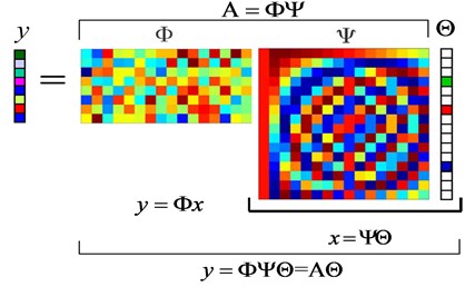
For vibration signal $\mathbf{x}\in {\mathbf{R}}^N$, our research will mainly focus on how to achieve bearing fault detection based on compressed sensing just using the compressive measurements $\mathbf{y}\in {\mathbf{R}}^M$ ($M<N)$ directly.

3. Bearing fault detection method

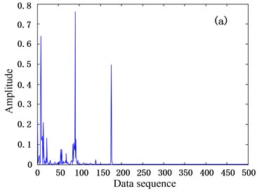
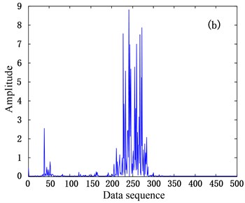
A practical bearing vibration signal (data source from [12], 6205-2RS JEK SKF deep groove ball bearing, with 12 K sampling frequency, 1797 r/min and 1 $HP$ load) in time domain can be denoted as $\mathbf{x}\in {\mathbf{R}}^N$ ($N=$1000). Using the discrete Fourier transform matrix as dictionary matrix $\mathrm{\Psi }$ and according to $\mathrm{\Theta }=\mathrm{\Psi }\mathbf{x}$, we can acquire the sparse representation coefficient $\mathrm{\Theta }$. Then the distribution of the elements in $\mathrm{\Theta }$ can reflect the energy distribution of the elements in signal $\mathbf{x}$ in frequency domain. The bearing vibration signals corresponding to different states should have different $\mathrm{\Theta }$. Considering $\mathrm{\Theta }$ is a complex vector, we calculate the square values of modulus of each element in $\mathrm{\Theta }$ and constitute vector $\tilde{\mathrm{\Theta }}$ in token of the energy distribution in $\mathrm{\Theta }$, as shown in Fig. 3 (due to the symmetry of $\tilde{\mathrm{\Theta }}$, we just plotted the half of the vector $\tilde{\mathrm{\Theta }}$ from 1 to 500 in data sequence). It can be seen from Fig. 3 that the distributions corresponding to the two different states (normal state and inner race state) differ obviously. Actually, the states of outer race fault and rolling ball fault also have the similar differences from the normal state. In general, the energy distributions corresponding to the same type of bearing state should be similar and invariable, which can be used to achieve fault detection.

Fig. 3The distributions of Θ~ corresponding to different bearing states, a) corresponding to normal state and b) corresponding to inner race fault state (the fault is single point, which is introduced to the bearing using electro-discharge machining with fault diameter of 0.021 inches and fault depth of 0.011 inches)

a)

b)

Compared to the original signal $\mathbf{x}\in {\mathbf{R}}^N$, we can acquire fewer compressive measurements $\mathbf{y}\in {\mathbf{R}}^M$ based on compressed sensing. According to the analysis previously, if we can estimate the distribution of $\mathrm{\Theta }$ in Eq. (4) with these fewer measurements directly, then bearing fault detection would be achieved. The energy distribution in $\mathrm{\Theta }$ can be described by the intervals which covered the elements with bigger modulus values in $\mathrm{\Theta }$. So the key of the proposed method is how to estimate the energy distribution of the elements in $\mathrm{\Theta }$ with measurements $\mathbf{y}$ directly. In the next several sections, we will introduce this fault detection method based on compressive measurements in detail.

4. Experimental tests

We will test the proposed method using vibration data corresponding to different states based on 6205-2RS JEK SKF deep groove ball bearings (data source from [12], signal sampling frequency is 12 K). All the vibration signals used in our test will be divided into lots of samples, and each sample can be denoted by $\mathbf{x}\in {\mathbf{R}}^N\text{,}$$N=$1000. In learning section, 840 samples corresponding to normal state will be used as training samples, which can be classified into four types. Each type has different motor load and motor speed when sampling. The training samples are shown in Table 1.

Choosing discrete Fourier transform matrix as dictionary matrix $\mathrm{\Psi }$ ($N$×$N$, $N=$ 1000), so the whole range should be $\mathcal{Z}=\left[\text{1;}\text{1000}\right]$. According to the interval learning method in Section 3.1 and setting the threshold $\epsilon$ as 0.9, the intervals corresponding to normal state and fault state can be determined as $\mathcal{T}=\left[\text{1; 177}\right]\cup \left[\text{825; 998}\right]$ and $\mathcal{F}=\left[\text{178; 824}\right]\cup \left[\text{999; 1000}\right]$respectively. Meanwhile, the number of the support points will be set as$k=\text{30}$.

The original test samples contained 840 normal state samples and 480 fault state samples, and both patterns can be classified into four types. Each type has different motor load and motor speed when sampling. The original test samples are shown in Table 2. The fault was designed as single point in inner race, which was introduced to the test bearings using electro-discharge machining with fault diameter of 0.021 inches and fault depth of 0.011 inches.

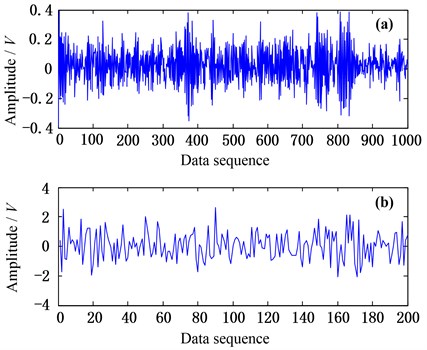
In practice, we should sample compressive measurements directly from practical analog signal. While we just focus on how to use these measurements to detect faults, so in our test the compressive measurements can be acquired by compressed sampling to original test samples mentioned above. We choose the observation matrix $\mathrm{\Phi }$ as Gaussian random matrix with dimensions as $M$×$N$$(M<N)$ [15-17]. This indicates that we can collect $M$ compressive data points in compressed sampling way during the same sampling time with that we collected $N$ data points in traditional sampling way. Then we can acquire 1320 compressive measurements with dimensions as $M$ which including 840 measurements corresponding to normal state and 480 measurements corresponding to fault state. For instance, some $N$-dimensional original test sample ($N=$1000, fault state) and the corresponding $M$-dimensional compressive measurements ($M=$200) with Gaussian random observation matrix $\mathrm{\Phi }$ are shown in Fig. 4.

Fig. 4General view of test data, a) is original test sample, b) is the compressive measurements corresponding to a)

The test result can be described using fault detection rate and false alarm rate. The fault detection rate characterizes the ratio of the number of the samples identified as fault state accurately to the number of all the fault samples used in test. The false alarm rate describes the ratio of the number of the samples recognized as fault state which actually should be normal state to the number of all the normal samples used in test. According to the analysis mentioned above, detection rate and false alarm rate should be affected by $M/N$, threshold $\delta$ and energy rate $\alpha$, which will be analyzed next respectively. To avoid the instability caused by the randomness of Gaussian random observation matrix $\mathrm{\Phi }$, the tests will be repeated several times and we use the average value as the final detection result.

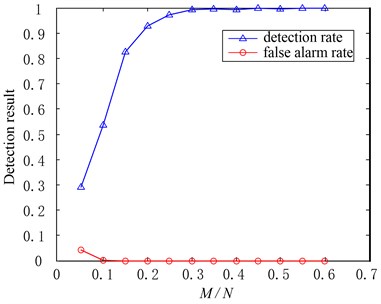
The detection result is shown in Fig. 5 when $\delta =\text{0.9}$ and $\alpha =\text{0.2}$ with the $M/N$ changes. It can be seen that with the increasing of measurements, the false alarm rate will fall to zero quickly and the detection rate will increase gradually until stabilization. This result should be consistent with the compressed sensing theory, for the increasing of measurements means that the condition information contained in compressive measurements will be enriched, which is of benefit to the fault detection.

Fig. 5Effects of M/N to the fault detection result when δ=0.9, α=0.2

The detection result is shown in Fig. 6 when $M/N=0.1\mathrm{}$ and $M/N=\text{0.2}$ and $\alpha =\text{0.2}$ with the threshold $\delta$ changes. It can be seen that in both cases with different $M/N$, with the increasing of the threshold $\delta$, both the detection rate and the false alarm rate will decline gradually. It should be noticed that the threshold$\mathrm{}\delta \mathrm{}$characterizes the ratio of the energy of the support points falling into interval $\mathcal{F}$ to the gross energy of all the support points recovered. So the bigger the threshold $\delta$ is, the more difficult the support points entering into the target interval $\mathcal{F}$ will be, and that’s why the fault detection rate and false alarm rate will decline.

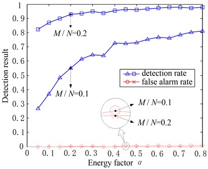
The detection result is shown in Fig. 7 when $M/N\text{=}\text{0.1}$ and $M/N=\text{0.2}$ and $\delta =\text{0.9}$ with the energy factor $\alpha$ changes. It can be seen that in both cases with different $M/N\mathrm{}$, the false alarm rate is always in a lower level closing to zero, and with the increasing of the energy factor $\alpha$, generally speaking, the detection rate will increase gradually.

Compared to the case with small number of measurements, we can see that the detection result using more measurements have less effect by the threshold $\delta$ and the energy factor $\alpha$ from Fig. 6 and Fig. 7. It also indicates the fact in Fig. 5 that the more measurements we use, the better the detection result will be. Therefore, we should sample more measurements as far as possible if the data storage and transmission permit.

Fig. 6Effects of δ to the fault detection result when M/N =0.1 and M/N=0.2, α=0.2

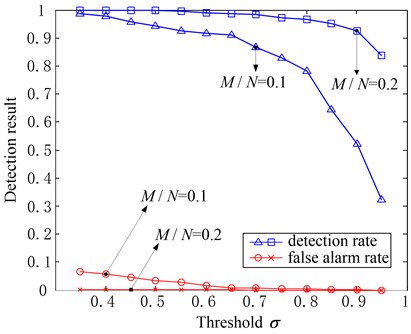
Fig. 7Effects of α to the fault detection result when M/N =0.1 and M/N=0.2, δ=0.9

In the above test, the fault corresponding to the test samples we used is single point fault with diameter of 0.021 inches and fault depth of 0.011 inches in inner race. For comparing the fault detection results in the cases with different levels of fault, we will use 480 fault samples corresponding to the case with low-level fault, and each sample can be denoted by $\mathbf{x}\in {\mathbf{R}}^N$, $N=$1000. Here the fault is single point fault with diameter of 0.007 inches (fault depth kept as 0.011 inches) in inner race. As with the above testing, we divide these fault samples into four types according to motor load and motor speed when sampling (same as that in Table 2). Each type includes 120 samples. Setting $k=\text{30}$, $\delta =\text{0.9}$ and $\alpha =\text{0.2}$, the fault detection rates with different number of measurements are shown in Fig. 8.

Fig. 8Detection rates for different level of faults (δ= 0.9, α= 0.2, M/N changes)

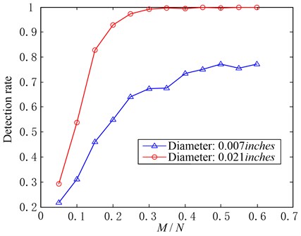
The false alarm rates are calculated using normal state samples, which should be invariable with the same parameters. So the false alarm rates in current condition will be the same as that shown in Fig. 5 and will not be shown in Fig. 8. It can be seen from Fig. 8 that in the case with the same $M/N\mathrm{}$, the detection rate corresponding to the case with fault diameter of 0.021 inches is higher than that with fault diameter of 0.007 inches. This result is in accord with that in theoretic case. In theoretic case, the severer the fault is, the more significant the differences of energy distributions between normal state signal and fault state signal in frequency domain will be. This is the foundation of the proposed method. So it shows the trend in Fig. 8 that the severer the fault is, the higher the detection rate will be.

The faults corresponding to all the test samples we used in above test are inner race faults. To validate the method in different fault patterns, we will use the samples corresponding to rolling ball fault and outer race fault. The two patterns of the faults are also single point faults with diameter of 0.021 inches and depth of 0.011 inches in bearing rolling ball and outer race respectively. Similar to the above test, there are 480 samples (each sample can be denoted by $\mathbf{x}\in {\mathbf{R}}^N$, $N=$1000) for each pattern, which can be divided into four types according to motor load and motor speed when sampling (same as that in Table 2). The fault detection results with different number of measurements are shown in Fig. 9 when $k=\text{30}$, $\delta =\text{0.9}$ and $\alpha =\text{0.2}$. The false alarm rates corresponding to different patterns are the same as that in Fig. 5, so they are not plotted. It can be seen from Fig. 9 that the detection rates will increase gradually in general until stabilization with the increasing of the measurements for every fault pattern. In the cases with inner race fault and outer race fault, the fault detection rate can reach to 95 %. While for the case with rolling ball fault, the detection rate will not be desirable which just around 60 %. The posture change of rolling ball should be complex in bearing operation, and this may result in the energy decentralization in frequency domain, so the detection rate to rolling ball fault using the proposed method will not be very high.

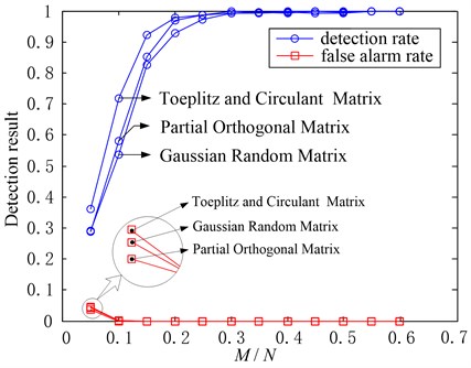
In the experimental tests of this section, we used the compressive measurements based on Gaussian random matrix. Actually, we can also use other compressed sampling ways. To validate our proposed method with different compressed sampling ways, we will compare the fault detection results in several typical compressed sampling ways (based on Gaussian random matrix, partial orthogonal matrix and Toeplitz and circulant matrix separately). In this test, we set $N=$ 1000, $\delta =\text{0.9}$, $\alpha =\text{0.2}$ and use the samples in Table 2 as the original test samples, then the fault detection results with different number of measurements ($M$) are shown in Fig. 10. It can be seen from Fig. 10 that all the three compressed sampling ways can achieve fault detection very well and can be used when collecting compressive measurements. While considering the higher computational efficiency and universality of Gaussian random matrix, and that’s why we used the Gaussian random matrix in the previous tests.

Fig. 9Detection rates corresponding to different fault patterns (δ=0.9, α=0.2, M/N changes)

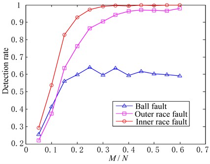
Fig. 10Fault detection results in three typical compressed sampling ways (δ=0.9, α=0.2, M/N changes)

5. Conclusions

In the process of condition monitoring, it is always necessary to monitor the component uninterruptedly for a long period of time. This process will generate masses of original data which will burden the storage and transmission. For this issue, we proposed a fault detection method based on compressed sensing, which can achieve fault detection directly using fewer compressive measurements compared to original data. Amount of samples corresponding to different bearing states were used to validate the method. The test results showed that with the increasing of the measurements, fault detection rate would increase and false alarm rate would decrease gradually. Meanwhile, the severer the fault was, the better the detection result would be. It is also indicated that the detection results will be better for inner race fault and outer race fault than that for rolling ball fault using our proposed method. The further research will focus on how to improve the fault detection result and how to achieve fault classification based on compressive measurements directly.