Abstract
Accurate estimate of the modal parameters of a structure is crucial to many practical engineering problems, such as finite element model updating/validation, damage detection, etc. As the measured data are inevitably contaminated by noise, accurately estimating modal parameters has been a difficult task. This article proposes an extended Prony’s method, which includes model order determination and noise reduction procedures before implementing the classical Prony’s method to estimate the modal frequencies and damping ratios for a jacket type offshore platform. In determining the model order, singular value decomposition (SVD) of a Hankel matrix, together with a model order indicator is applied. For removing noise from the measured signal to yield a filtered signal with a known model order, a structured low rank approximation (SLRA) method for the Hankel matrix is carried out. To validate the applicability of the proposed approach, experimental studies based on a steel model of jacket type offshore platform were firstly performed. Using measured data from four accelerometers mounted at different locations of the test model, it is found that the modal parameters including translational mode (x or y direction) and torsional mode estimated from the filtered signals of the four locations separately are in excellent agreement. Using sea test data measured from accelerometers mounted at two different locations of the test platform, it is also found that the modal parameters estimated from the filtered signals of the two locations separately are in excellent agreement. It is concluded that the proposed approach is very accurate on estimating the modal parameters. A significant improvement can be achieved when the filtered, rather than the originally measured, signals are used.
1. Introduction
Steel jacket type platforms as the most common kind of offshore structures have been widely used in offshore oil and gas exploitation. During the service life, the continuous ageing and subsequent structural deterioration of an offshore structure may cause the change on its mass and/or stiffness distribution. Consequently, the modal properties of the structure, such as natural frequencies, damping ratios and mode shapes, may alter as well. Modal parameter estimation is the process of determining modal parameters from experimental data [1]. Accurate estimate of the modal parameters, in addition to being utilized in a typical modal-based damage detection method, can also provide a basis for finite element updating and validation [2, 3].
Conventional modal identification techniques employed in laboratories are often based on estimating a set of frequency response functions (FRFs), or on the corresponding impulse response functions (IRFs), relating the applied force (input) and corresponding response (output) at several pairs of points along the structure with enough high spatial and frequency resolution. Extracting modal parameters from measurements has been a subject of constant improvement and enhancements, and the reader is referred to the subject textbooks for a detailed treatise on various modal identification methods [4, 5]. The modal parameters of civil structures, however, are often necessary to be estimated exclusively from output signals because dynamic testing of large civil structures, such as jacket type offshore platforms, can only be performed in the field and the applied excitation force is usually not achieved for technically and/or economically prohibited.
Measured signals are inevitably contaminated with noise when a data acquisition system is used for an experimental measurement, the measured FRF and IRF may not be clean enough for estimating the modal parameters with proper accuracy [6]. In the modern modal analysis, it does not seem to have a particular procedure intending to eliminate the noise. In fact, the computational model order is often set higher than the true system order, so the so-called “noise modes” could be absorbed [7]. The inclusion of a larger number than the critical number of model order will cause the creation of “computational” modes in addition to the genuine “physical” modes which are of interest.
In contrast to the classical ways – choosing a higher model order intentionally for absorbing noise – in the modal parameter estimation process, the proposed procedure is to firmly determine the model order and eliminate much noise from the measured IRF before applying a time domain technique for modal parameter estimation. In determining the model order, the first step is to construct a Hankel matrix based on the measured IRF. Then singular value decomposition (SVD) is applied, together with a model order indicator, to determine the rank of the Hankel matrix. This rank in theory is equal to two times the number of modes embedded in the measured IRF [8]. For removing noise from the measured IRF to yield a filtered IRF with a known model order, a structured low rank approximation (SLRA) method for the Hankel matrix must be carried out. Mathematically, the SLRA concerns the construction of the nearest approximation to a given matrix by a matrix with a specific rank and a specific linear structure [9-11]. In this case, the resulting matrix must maintain the Hankel structure, and be lowered in rank as well. The data matrix being Hankel structured is equivalent to the existence of a linear time-invariant system that fits the data and the rank constraint is related to a bound on the model order [8, 12]. Once the filtered IRF is obtained, the complex exponential method (Prony’s method) can be applied to extract the modal parameters [4, 5].
In this paper, the performance of the proposed method for jacket type offshore platform will be investigated using real measurements from an experimental model and a sea test platform. The measurements obtained by using accelerometers are employed to estimate the modal frequencies and damping ratios throughout the studies.
2. Model order determination and noise reduction
As the measured data are contaminated by noise, weak signals associated with certain modes are likely buried in the noise. Prior to noise reduction based on the SLRA method, the model order must be determined. In determining the model order, a Hankel matrix is constructed based on the measured signal, and then SVD is applied, together with a model order indicator, to determine the rank of the Hankel matrix. This rank in theory is equal to two times the number of modes embedded in the measured signal.
2.1. Rank of Hankel matrix
Let {hl}, l=0,1,2,…, represent an IRF sequence of an N degree of freedom (DOF) system, and be sequentially filled to form a rectangular Hankel matrix Hm×n, with m,n≥2N as:
The original sequence {hl} is readily retrieved from the first row and last column, or the first column and last row, of matrix Hm×n. Because an N-DOF dynamic system (with N simultaneous second-order linear differential equations) is mathematically equivalent to a linear differential equation of order 2N, the IRF sequence {hl} must satisfy a linear difference equation:
wheren=0, 1,…, and βm, m=0,⋯,2N-1 are real coefficients.
If {hl} is an exact (noise-free) IRF of an N-DOF dynamic system, then the rank of Hm×n should be equal to 2N, as long as m and n are both greater than or equal to 2N and all N modes contribute to the IRF. The above statement could be illuminated based on Eq. (2) as it is rewrited into a linear recursive form:
This recursive equation suggests that each term of the sequence is defined as a linear combination of the preceding 2N terms. Thus a discrete IRF of an N-DOF dynamic system can be fully described by any of its 2N consecutive values. Because only 2N independent values are possible in a discrete IRF, the rank of Hm×n constructed from {hl} cannot exceed 2N.
2.2. Rank determination from SVD
One common way of knowing the rank of a matrix is based on SVD of the matrix. Let the SVD of a matrix A∈Rm×n be expressed as:
where U∈Rm×m and VT∈Rn×n are orthonormal matrices, and Σ∈Rm×n is a rectangular diagonal matrix whose diagonal elements are singular values, arranged in order of deceasing size. Because some of the singular values may be zero, Σ can be partitioned into a submatrix Σr of r nonzero singular values and several zero matrices as:
where Σr is a r×r diagonal matrix. The decomposition then becomes A=UΣVT=UrΣrVTr, where Ur and Vr consist of the first r columns of U and V. This decomposition indicates the rank of A is r. For theoretical data, the singular values should go to zero when the rank of the matrix is exceeded. For measured data, however, due to random errors and small inconsistencies in the data, the singular values will not become zero but will become very small.
2.3. Corrupted IRF and its Hankel matrix
When a measured IRF sequence {hl} is contaminated by random noise, it can be expressed as:
where and represent the true signal and noise, respectively, and is the number of DOF that is necessary to represent the measured data. Because some modes might not contribute to this particular IRF, is possible less than , the number of DOF of the system.
Theoretically, the Hankel matrix corresponding to the noisy signal in Eq. (6) can be partitioned into two parts:
where and represent Hankel matrices associated with the uncontaminated signal and noise parts, respectively. Because the signal {} is contributed by modes, its corresponding Hankel matrix must be with a rank . A noise elimination method for estimating {} from is thus by estimating based on , where the estimate of , denoted , must be a Hankel matrix with rank . While approximating to its “nearest” matrix , an often used criterion is based on minimizing the Frobenius norm of the difference between and , denoted [11].
2.4. Unstructured low rank approximation
The unstructured low rank approximation problem is to approximate a data matrix with another matrix that has a specific lower rank by minimizing , and the unstructured matrix can be obtained via the truncation of the SVD of the data matrix . This approach has often been referred to as based on the truncated singular value decomposition (TSVD) technique or Eckart-Young theorem [13], which is summarized below.
Given an matrix of dimensions × of rank where and its singular value decomposition:
then there exists an × matrix of rank which minimizes when:
where is the same matrix as except that it contains only the largest singular values, i.e., the other singular values are replaced by zeros.
2.5. Cadzow’s algorithm
The optimal Frobenius norm lower rank approximation to a given Hankel matrix can be obtained from the TSVD of , but the resulting matrix will not possess a Hankel structure. In mathematical terms, the noise reduction problem here is a structured low rank approximation problem. In addition to lower its rank, the resulting matrix must maintain a Hankel structure. A simple engineering algorithm for the restoration of a Hankel matrix is the iterative Cadzow’s algorithm, which has been also called the anti-diagonal averaging method [12, 14]. It can be summarized by the following steps:
1) Use the TSVD technique with an appropriate value of rank estimated from the data to obtain a low rank approximation to the Hankel data matrix. Note that the resulting matrix will not be a Hankel matrix.
2) Rebuild a Hankel matrix from by replacing all elements of each anti-subdiagonal by the arithmetic average of the elements along the anti-subdiagonal. Note that the resulting Hankel matrix will not be rank .
In Cadzow’s algorithm, the low rank approximation and anti-subdiagonal averaging are alternated iteratively until a convergence test has been met. It has been proven that such iterative usage always converges [14, 15].
3. Experimental studies
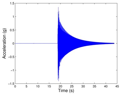
The effectiveness of the proposed method will be ultimately evaluated based on field test data. However, in order to verify the correctness of the developed algorithms, also to provide insight for analyzing field test data, the experimental measurements in laboratory will be investigated firstly. The experimental model of a jacket type offshore platform is shown in Fig. 1, where the sensors are mounted at the key nodes of the model. Four accelerometers are selected for the studies, which are mounted at and directions of nodes 1 and 2, respectively. Exciting at the location of node 3 (corner of the deck) from and directions by an impulsive load, respectively, so the translational modes ( or direction) and torsional modes can be extracted from the corresponding recorded acceleration signals (, , and ). and are -direction responses of nodes 1 and 2 from -direction excitation of node 3, respectively; and are -direction responses of nodes 1 and 2 from -direction excitation of node 3, respectively. Fig. 2 is the IRF of for about 45 seconds with sampling rate 200 Hz. However, only the segment between 23 and 25.555 seconds with 512 sample points of each IRF would be taken for the later analysis, respectively.
Fig. 1The experimental model of a jacket type offshore platform and the sensors mounted
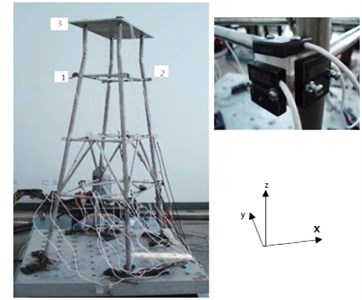
Fig. 2Measured IRF of S1x
3.1. Model order determination
Determining the model order of an IRF is by estimating the rank of its related Hankel matrix. For an IRF with 512 steps, the corresponding largest (nearly square) Hankel matrix is constructed, for convenience and without losing generality.
For a response signal contributed only by modes, the rank of the Hankel matrix should be , which is twice the number of modes contained to the signal. Estimating the rank of a matrix could be easily done if the singular values of the matrix have been ordered sequentially from the largest to the smallest. A model order indicator () is introduced, which is defined as the relative change ratio of the decreasing singular values, denoted:
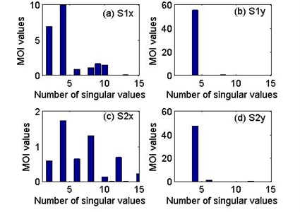
where , is the singular value, and the maximum change ratio corresponds to the model order. The model order indicators associated with the Hankel matrices for four IRFs can be calculated by using Eq. (10) and are plotted in Fig. 3, from which it can be seen that the maximum values for the four Hankel matrices corresponding to the model orders are 4, respectively.
Fig. 3Model order indicators of the four Hankel matrices related to: (a) S1x, (b) S1y, (c) S2x and (d) S2y
3.2. Noise elimination
The model orders of the four IRFs have been determined equal to 4 (see Fig. 3). In this section, Cadzow’s algorithm is applied to demonstrate the performance of the noise elimination below.
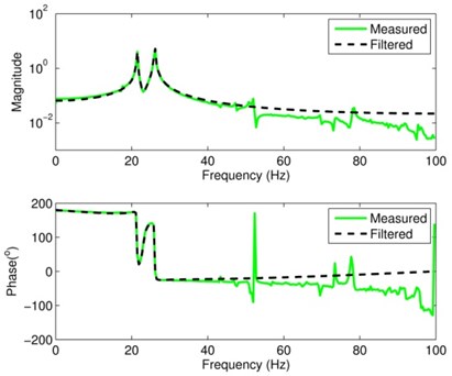
Fig. 4Comparison of the measured and filtered FRFs of signal S1x
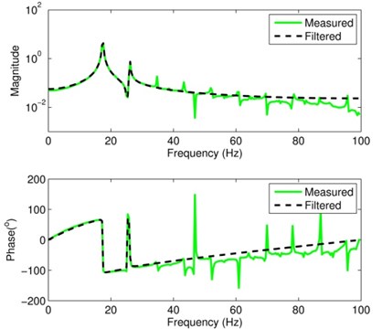
Cadzow’s algorithm alternates iteratively between two steps: unstructured low rank approximation (via TSVD technique) and anti-subdiagonal averaging. Working on the Hankel matrix , which is the maximal size for an IRF with 512 samples, an excellent result of the noise elimination can be obtained. The measured FRF and the corresponding filtered FRF associated with are shown in Fig. 4. The filtered FRF has 2 sharp peaks within the frequency range 0-100 Hz, and the visible level of noise at the measured FRF has been successfully eliminated. Similarly, Fig. 5 shows the measured and filtered FRFs associated with , and the noise elimination from the measured FRF appears to be very good also. The performances of noise elimination associated with and are also good which are not listed in the form of figures here.
Fig. 5Comparison of the measured and filtered FRFs of signal S1y
3.3. Modal parameters identification
After carrying out the noise elimination to obtain the filtered IRFs, Prony’s method is applied for estimating modal parameters. The first three modal frequencies identified from the measured and filtered signals are listed in Table 1. Their counterparts computed from a finite element model (FEM) are also included for comparison. Because the directions of excitation are and at node 3 (corner of the deck), and response locations are also and directions of node 1 and node 2, translational mode ( or direction) and torsional mode can be identified from each signal. The three modal frequencies obtained from the experimental data basically agree with those of the FEM, recognizing that discrepancy always exists between the true physical structure and its FEM. Modal frequencies are global parameters and theoretically they should remain the same when they are estimated from different IRFs. Due to a lack of the true values for the modal frequencies of the test structure, examining the agreement among the modal frequencies estimated from different signals seems to be the most logical way to evaluate the estimation performance. As exhibited in Table 1, the corresponding modal frequencies identified from the filtered IRFs associated with and , and are in excellent agreement.
Table 1The first three modal frequencies identified from the measured and filtered signals
Mode | FEM (Hz) | (Hz) | (Hz) | (Hz) | (Hz) | ||||
1 | 17.207 | 17.363 | 17.471 | – | – | 17.584 | 17.471 | – | – |
2 | 21.581 | – | – | 21.647 | 21.798 | – | – | 21.831 | 21.798 |
3 | 26.350 | 24.961 | 26.520 | 26.739 | 26.523 | 26.647 | 26.520 | 26.325 | 26.523 |
The subscript “” and “” stand for “measured” and “filtered”, respectively. | |||||||||
Shown in Table 2 are the values for the damping ratios of the first three modes identified from the measured and filtered IRFs. The damping ratios identified from the measured signals are poor. In particular at , and there are negative quantities which are physically impossible. Compared with the identified values from the measured signals, the damping ratios identified from the filtered signals seem reasonable as they are also in excellent agreement. The results also indicate that the improvement of estimating damping ratios from using filtered IRF (instead of measured IRF) is more significant than that of modal frequencies.
Table 2The first three damping ratios identified from the measured and filtered signals
Mode | (%) | (%) | (%) | (%) | ||||
1 | 0.10259 | 0.12151 | – | – | 0.10595 | 0.12159 | – | – |
2 | – | – | –0.34202 | 0.17692 | – | – | –0.21741 | 0.17676 |
3 | 0.55338 | 0.14237 | 0.17862 | 0.14212 | –0.06919 | 0.14249 | 0.38668 | 0.14227 |
The subscript “” and “” stand for “measured” and “filtered”, respectively. | ||||||||
In performing experimental modal analysis, over-determined models have been often used, and stability diagrams have been routinely plotted to eliminate spurious numerical poles (modes). When producing a stability diagram, the poles corresponding to a certain model order are compared to the poles of a one order-higher model [16]. If the pole (modal frequency, damping ratio and modal vector) differences are within preset limits, the pole is labeled as a stable one. Adopting the preset limits with 1 % difference for frequencies, 5 % for damping ratios, and 2 % for the modal vector among two consecutive model orders, namely:
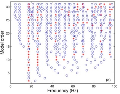
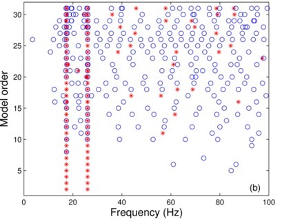
where and denote an estimated frequency, damping ratio and modal vector, respectively, with model order ; and “∙” is the inner product operation. The stability diagrams can be plotted based on the measured and filtered signals of by choosing the model orders ranging from 2 to 31, which is shown in Fig. 6. Although the stability diagram associated with the measured signal has consistent frequency estimates near the two system frequencies (17.471 Hz and 26.520 Hz) extending from lower order to higher order models, many poles have been labeled unstable (“o”) because they did not meet the preset stability standard. In contrast, the stability diagram associated with the filtered signal has consistent and stable poles (“*”) all the way from models with order 2 to 31.
Fig. 6Stability diagrams corresponding to: (a) measured, and (b) filtered signals of S1x. The used symbols are: “o”, not stable; “*”, stable frequency, damping and modal vector
a)
b)
4. Field data studies
Now, the performance of the proposed method is examined using the sea test data. As the test platform has been built for many years, its modal properties might have been changed from its original state due to various reasons, such as structure deterioration, marine growth, etc. In addition, the modal properties of an offshore structure in water would be significantly different from those in air. The focus of this study is on examining the proposed method for estimating modal parameters from measured acceleration signals of the test platform.
The test structure is a four-leg jacket type offshore platform located in Bohai Sea, China (see Fig. 7). The plane dimension is about 16 m×11 m at the deck elevation, which is 10.0 m above the still water level. The elevation (with reference to the still water level) of the three stories are at +4.0 m, –2.0 m and –9.0 m, respectively. The four sloping legs (with inclination 10:1) are cylindrical piles with uniform outer diameter 1.34 m and wall thickness 0.025 m. The horizontal braces at elevations +4.0 m and –2.0 m are with 0.61 m and 0.02 m, and those at elevation –9.0 m with 0.61 m and 0.018 m. Vertical braces between elevations –2.0 m and –9.0 m are with 0.4 m and 0.014 m.
Fig. 7The test jacket platform at Bohai Sea in China
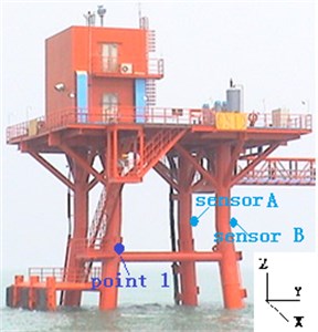
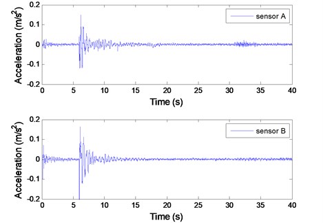
The sea test data were collected based on the step relaxation procedure. The test platform was pulled by a boat at point 1 (see Fig. 7) in -direction. After a static displacement of the test structure was reached, the test structure was released and relaxation response accelerations related to two accelerometers oriented in the -irection, termed sensors A and B, with sampling frequency 200 Hz were recorded. The two recorded acceleration signals are shown in Fig. 8.
Fig. 8Measured acceleration signals from sensors A and B
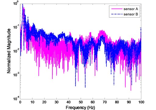
While conducting Prony’s method, only the segment between 7 s and 12.12 s of each measured signal, with 1024 sample points, is to be used. Shown in Fig. 9 are the corresponding Fourier spectra of the two segments. It is found that the two recorded signals all contain significant random noise, and it is difficult to estimate the modal frequencies by using the simple peak-picking method.
Fig. 9Fourier analysis of the two measured segmented signals
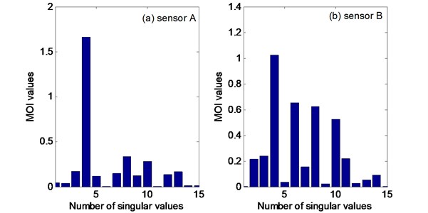
To determine the model order of each measured signal, the s of the Hankel matrices associated with the two segmented signals are plotted (see Fig. 10). It is found that the maximum values for the two Hankel matrices corresponding to the model orders are 4. Carrying out Prony’s method with the model order 4, and using the measured (unfiltered) signals for sensors A and B, the consistent, physically meaningful estimates for modal frequencies and damping ratios could not be obtained. This confirms that the classical Prony’s method is sensitive to noise and would not be recommended for analyzing noisy signals without purposely increasing model order to absorb noise.
Fig. 10Model order indicators of the two Hankel matrices related to sensors A and B
After filtering the measured signals by performing the SLRA to make the rank of the related Hankel matrices equal to 4, the Fourier spectra of the two filtered signals are shown in Fig. 11. The filtered signals become smoother and they have 2 spectral peaks, and agree with each other well, as expected.
Implementing Prony’s method for the filtered signals yields the estimated frequencies and damping ratios listed in Tables 3. All 2 estimated frequencies from each sensor agree very well, all with relative error less than 0.2 %, a dramatic improvement over using the measured (noisy) data directly. The relative errors of the first and second estimated damping ratios are larger: 1.49 % and 2.21 %, respectively. However, these errors are acceptable because the corresponding damping ratios are very small.
Fig. 11Fourier analysis of filtered signals at sensors A and B
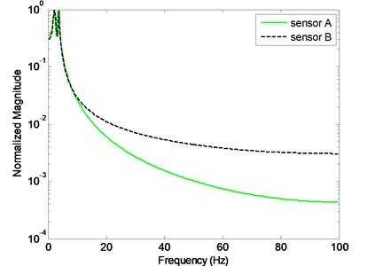
Table 3Estimated frequencies and damping ratios from the filtered signals of sensors A and B
Mode | Frequencies (Hz) | Relative difference | Damping ratios | Relative difference | ||
Sensor A | Sensor B | Sensor A | Sensor B | |||
1 | 2.0866 | 2.0888 | 0.11 % | 0.0134 | 0.0136 | 1.49 % |
2 | 3.6261 | 3.6329 | 0.19 % | 0.0272 | 0.0266 | 2.21 % |
5. Concluding remarks
Due to the noise and the uncertainty of the number of modes (or model order) in measured signals, accurately estimating modal parameters has been a challenging task. Traditional method to improve modal parameter estimation is by purposely over specifying the computational model order to absorb noise; however, sorting out computational modes (noise modes) is still a difficult task. It requires experience and judgment to use sorting tools (such as stability diagrams) effectively. An extended Prony’s method, which includes model order determination and noise reduction procedures before implementing the classical Prony’s method, was proposed in this article. Basically, the proposed approach intends to use the actual system order as the computational model order and rejects much noise prior to performing the modal parameter estimation. The proposed method included three steps: (1) determining the rank of a Hankel matrix associated with the measured IRF based on SVD, together with the model order indicator, where the rank is theoretically twice the number of modes contributing to the measured IRF, (2) implementing Cadzow’s algorithm for the SLRA on the Hankel matrix to achieve the noise removal from the measured IRF to obtain a filtered IRF, and (3) using Prony’s method to estimate the modal parameters from the filtered IRF with a known model order.
The efficiency of the proposed method for a jacket type platform was evaluated based on an experimental model in laboratory and a field test. Although the true values of the modal parameters of the test structures were not known, it could still be judged the performance of the proposed scheme based on examining the agreement among the modal parameters estimated from IRFs measured from the accelerometers mounted at different locations of the test structures. Carrying out the proposed method, it was found that the modal parameters identified from the filtered IRFs associated with the different accelerometers were in excellent agreement.
References
-
Richardson M., Schwarz B. Modal parameter estimation from operating data. Sound and Vibration, Vol. 37, Issue 1, 2003, p. 28-36.
-
Li H. J., Wang J. R., Hu S-L. J. Using incomplete modal data for damage detection in offshore jacket structures. Ocean Engineering, Vol. 35, Issue 17-18, 2008, p. 1793-1799.
-
Wang S. Q. Damage detection in offshore platform structures from limited modal data. Applied Ocean Research, Vol. 41, Issue 2013, 2013, p. 48-56.
-
Ewins D. J. Modal testing: theory, practice and applications. Research Studies Press, Baldock, Hertfordshire, England, 2000.
-
Maia N. M. M., Silva J. M., He J., Lieven N. A. J., Lin R. M., Skingle G. W., To W. M., Urgueira V. A. P. Theoretical and experimental modal analysis. Research Studies Press, Taunton, Somerset, England, 1997.
-
Sanliturk K. Y., Cakar O. Noise elimination from measured frequency response functions. Mechanical Systems and Signal Processing, Vol. 19, Issue 3, 2005, p. 615-631.
-
Allemang R. J., Brown D. L. A unified matrix polynomial approach to modal identification. Journal of Sound and Vibration, Vol. 211, Issue 3, 1998, p. 301-322.
-
Markovsky I., Huffel S. V. Overview of total least squares methods. Signal Processing, Vol. 87, Issue 10, 2007, p. 2283-2302.
-
Markovsky I. Structured low-rank approximation and its applications. Automatica, Vol. 44, Issue 4, 2008, p. 891-909.
-
Schuermans M., Lemmerling P., Huffel S. V. Block-row hankel weighted low rank approximation. Numerical Linear Algebra with Applications, Vol. 13, Issue 4, 2006, p. 293-302.
-
Chu M. T., Funderlic R. E., Plemmons R. J. Structured low rank approximation. Linear Algebra and its Applications, Vol. 366, 2003, p. 157-172.
-
Cadzow J. A. Signal enhancement – a composite property mapping algorithm. IEEE Transactions on Acoustics, Speech, and Signal Processing, Vol. 36, Issue 1, 1988, p. 49-62.
-
Eckart G., Young G. The approximation of one matrix by another of lower rank. Psychometrika, Vol. 1, Issue 3, 1936, p. 211-218.
-
Tufts D., Shah A. Estimation of a signal waveform from noisy data using low-rank approximation to a data matrix. IEEE Transactions on Signal Processing, Vol. 41, Issue 4, 1993, p. 1716-1721.
-
De Moor B. Total least squares for affinely structured matrices and the noisy realization problem. IEEE Transactions on Signal Processing, Vol. 42, Issue 11, 1994, p. 3104-3113.
-
Peeters B. System identification and damage detection in civil engineering. Ph. D. thesis, Katholieke Universiteit Leuven, 2000.
About this article
This study was supported by the National Natural Science Foundation of China (Grant No. 51309239), the Shandong Provincial Natural Science Foundation, China (Grant No. ZR2011EEQ022), the Qingdao Plan of Science and Technology Development, China (Grant No. 13-1-4-216-jch) and the Fundamental Research Funds for the Central Universities.
